It’s Wednesday and I just finished a ‘Conversation’ with the Economics Society of Australia, where I talked about Modern Monetary Theory (MMT) and its application to current policy issues. Some of the questions were excellent and challenging to answer, which is the best way. You can view an edited version of the discussion below and…
Aggregate Demand Part 3
I am now using Friday’s blog space to provide draft versions of the Modern Monetary Theory textbook that I am writing with my colleague and friend Randy Wray. We expect to complete the text by the end of this year. Comments are always welcome. Remember this is a textbook aimed at undergraduate students and so the writing will be different from my usual blog free-for-all. Note also that the text I post is just the work I am doing by way of the first draft so the material posted will not represent the complete text. Further it will change once the two of us have edited it.
[NOTE: THIS CONTINUES THE CHAPTER ON AGGREGATE DEMAND]
Which generates what we call the equilibrium national income equation:
(8.11) Y = 1/(1 – c(1 – t))[C0 + G]
You will notice that the equilibrium income that results from the sum of consumption and government spending is the product of two exogenous spending components, C0 + G and the coefficient 1/(1 – c(1 – t)), which we call the expenditure multiplier.
We sometimes refer to the exogenous spending components as autonomous spending because they do not depend on national income – they are given.
The expenditure multiplier tells us how much national income (Y) will change for a given change in autonomous spending
The expenditure multiplier is a ratio involving the marginal propensity to consume (c) and the marginal tax rate (t). By inspection we can see that the higher is the MPC and the lower is the tax rate the larger will be the expenditure multiplier. The task now is to explain why that is the case in terms of the economic processes involved.
The Expenditure Multiplier
At present we continue to ignore private investment spending and also the impact of exports and imports. In the next section of this Chapter we will complete the picture and learn that open economies typically have lower expenditure multiplier values than more closed economies.
We start with the essential insight that aggregate demand drives output with generates incomes (via payments to the productive inputs). Accordingly, what is spent will generate income in that period which is then available for use. For example, workers who are hired by firms to produce goods and services spend the incomes they earn as do suppliers of raw materials and other inputs to the production process.
There are various ways in which the income derived from the payments arising from output production can be used. The income can be used for:
- Increased consumption.
- Increased saving.
- Relinquishing tax obligations to government.
In the next section, we will add a further use – the possibility of increased import spending.
Imagine that the tax rate is 0.20 and the marginal propensity to consume is 0.80, then for every dollar produced and paid out as income we know that the government will take 20 cents, and from the extra 80 cents of disposable income that is left, consumers will spend 64 cents and save 26 cents.
Note that the stream of income that follows expenditure on output does not fully cycle back into renewed income and expenditure. We say that some of the income leaks from the expenditure system via taxation and saving. So for a $1 produced only 64 cents is recycled back into expenditure in the next period with 36 cents leaking out of the system via taxation (20 cents) and saving (16 cents).
Take taxation first. When income is produced, the households end up with less than they are paid out in gross terms because the government levies a tax. So the income concept available for subsequent spending is called disposable income (Yd).
When households receive extra disposable income they then decide how much of it to consume. Consumers make decisions to spend a proportion of their disposable income and the marginal propensity to consume is the amount of each dollar they spent at the margin (that is, how much of every extra dollar to they consume). The residual that is not consumed is then lost to the expenditure system via private saving.
It is easy to see that for every $100 produced, the income that is generated and distributed results in $64 in consumption and $36 in leakages which do not cycle back into spending.
For income to remain at $100 in the next period, there has to be equal “injections” of expenditure from sources of demand that are independent of income – the exogenous or autonomous spending components – to offset the leakage of the $36 that is lost via saving and taxation.
In our model so far that injection might come from government spending but in the broadened model developed in the next section it could also come from investment and/or exports. These injections are seen as coming from “outside” the output-income generating process.
As we will see, GDP and national income is stable when the injections equal the leakages.
Now imagine that GDP has been stable at some level for some time. The question that the concept of the expenditure multiplier allows us to answer is: what would happen if government increased spending by, say, $100? By how much does output and income rise in response to increased aggregate demand?
In terms of how previous example, we already know that if national income changes by $100 there will be $64 of extra consumption expenditure, which is induced by the initial injection in spending. But the process of adjustment to that initial increase in national income of $100 does not stop there. What happens next?
The expenditure multiplier is defined as the total change in real income that results from a dollar change in exogenous aggregate demand. The total change in income is the result of a sequence of induced spending effects that are triggered by an initial injection of spending. The initial injection spreads across time and space as workers receive higher incomes and are motivated to increase their spending.
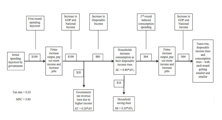
Figure 8.4 provides a graphical summary of the initial monetary flows that drive the expenditure multiplier process. In the example shown, the extra $100 in government spending, leads firms to produce more output and increase income payments by $100 (under the assumptions in this Chapter about the aggregate supply response).
Already you can understand that the initial spending increase of $100, which might have been a government order for new public school buildings, provides workers involved in the production of those buildings with increased incomes. These workers, then spend some of their income gains on various goods and services (for example, local shops, local service suppliers, goods and services from firms not in their local area etc).
As a result, the initial spending “fans out” or spreads throughout the entire economy. We say that the initial spending multiplies into a much larger increase in spending.
The initial recipients of the increased income pay the government an extra $20 in taxes and then increase consumption by $64 and save $36. The second-round spending which we called induced consumption then motivates the firms which enjoy the increase in demand for their goods and services to increase output and pay out an extra $64 in income.
That extra income is, in turn, the source of further increases in tax revenue for the government (0.20 by $64 = $12.80) and consumption (0.80 by $51.20 = $41.00) with saving also rising by the difference between the change in disposable income ($51.20) and the change in consumption ($41.00), that is, $10.20.
Notice that the second-round expenditure response to the initial injection of $100 is $64 and the third-round response is $41. Further, the tax revenue gained by government and the volume of saving also fall with each subsequent spending round.
This is because the subsequent induced consumption spending creates leakages at each stage which reduces the spending response in the next round.
Figure 8.4 The expenditure multiplier process

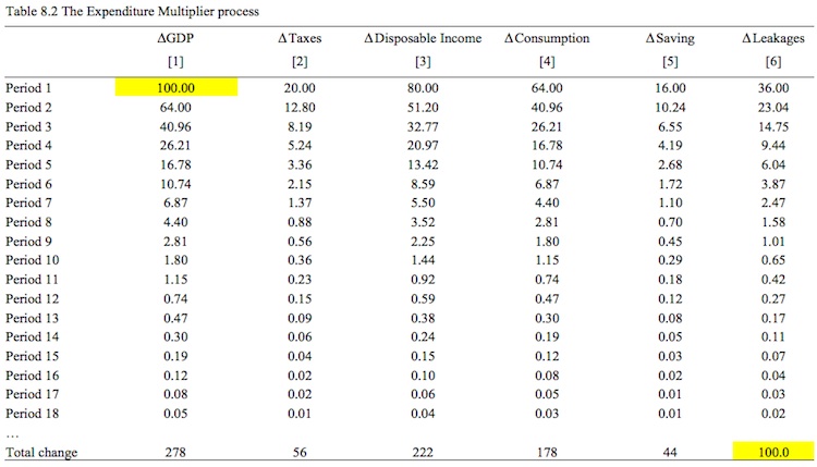
Table 8.2 shows the process for 18 periods (by which the induced consumption is near zero) and the final change in income that results from the initial rise in government spending by $100. In the resources available for this Chapter you will be able to download the spreadsheet and manipulate the initial expenditure injection, the tax rate and the marginal propensity to consume to produce your own simulations.
Note the Leakages are getting smaller with each spending period following the initial injection of $100. In the bottom row we see that the sum of all the period-by-period changes in GDP (Column [1]) equals $278. The total increase in tax revenue (Column [2]) is $56. The total increase in disposable income (Column [3]) is thus $222, which leads to total induced consumption (Column [4]) of $178 and the total increase in saving (Column [5]) is $44.
We define the multiplier as the total change in GDP for a one dollar initial increase in aggregate demand. The initial increase was $100 and the total change in GDP that it generated was $278. The multiplier is thus:
multiplier = δY/δG = $270/$100 = 2.78
Where δG was, in this example, the initial increase in aggregate demand. We can clearly generalise this to refer to any initial increase in autonomous demand (A).
The multiplier in our particular example is thus 2.78, which means that for every $1 of increased aggregate demand total GDP (and national income) will rise by $2.78.
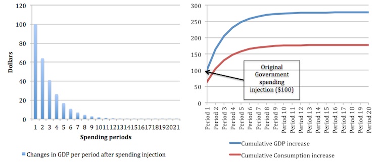
Figure 8.5 provides another perspective on the expenditure multiplier process. The left-hand panel plots the period-by-period changes in GDP (Column [1] in Table 8.2) following the initial injection of $100. The right-panel shows the cumulative increase for each period in GDP and Consumption.
You can see that the economy responds immediately to the initial injection of aggregate demand and as time passes and the subsequent induced consumption flows become smaller and smaller, the total response flattens and then exhausts once the leakages rise to equal the initial injection.
Figure 8.5 Changes in GDP and cumulative change in GDP for a $100 government spending injection

Changes in the Multiplier
In Equation (8.11) we defined the expenditure multiplier as 1/(1 – c(1 – t)), which means in that in a closed economy, its value depends on the marginal propensity to consume (c) and the tax rate (t). Given that the marginal propensity to save (s) is just (1-c), the multiplier is higher when the leakages – saving and taxation – a lower.
This is because the lower the leakages from each spending round, the larger is the induced consumption and the longer is the adjustment process following an initial injection of demand.
Figure 8.6 shows the impact of an increase in the marginal propensity to consume from 0.8 to 0.9. Households now consume 90 cents of every extra dollar in disposable income they receive.
The initial impact of the $100 government spending injection is identical but the second- and later round induced consumption effects are larger and therefore last long because the leakages in each period are smaller.
Figure 8.5 Changes in GDP and cumulative change in GDP for a $100 government spending injection

Conclusion
The next part of this Chapter will introduce investment and the net exports
Saturday Quiz
The Saturday Quiz will be back again tomorrow. It will be of an appropriate order of difficulty (-:
That is enough for today!
(c) Copyright 2012 Bill Mitchell. All Rights Reserved.

“… and from the extra 80 cents of disposable income that is left, consumers will spend 64 cents and save 26 cents.”
It must be 16 cents that are saved, of course. (The mistake does not have any consequences for the following calculations. Below, you state correctly that savings go up by 16 cents and continue to work with this correct number.)