It’s Wednesday and I just finished a ‘Conversation’ with the Economics Society of Australia, where I talked about Modern Monetary Theory (MMT) and its application to current policy issues. Some of the questions were excellent and challenging to answer, which is the best way. You can view an edited version of the discussion below and…
Keynes and the Classics Part 8
While I usually use Friday’s blog space to provide draft versions of the Modern Monetary Theory textbook that I am writing with my colleague and friend Randy Wray, today I am departing from that practice (deadlines looming) and devoting the next two days to textbook writing. We expect to complete the text during 2013 (to be ready in draft form for second semester teaching). Comments are always welcome. Remember this is a textbook aimed at undergraduate students and so the writing will be different from my usual blog approach.
I am currently working on Chapter 11 which opens like this:
Chapter 11
11.1 Introduction and Aims
In Chapter 10, we discussed issues relating to labour market measurement. In this Chapter we will focus on theoretical concepts that underpin the measurement of economic activity in the labour market and the broader economy.
The Chapter has five main aims:
- To explain why mass unemployment arises and how it can be resolved.
- To develop the concept of full employment.
- To consider the relationship between unemployment and inflation – the so-called Phillips Curve.
- To develop a buffer stock framework for macroeconomic management (full employment and price stability) and compare and contrast the use of unemployment and employment as buffer stocks in this context.
- To more fully explore the concept of a Job Guarantee (employment buffer stock) approach to macroeconomic management.
NOTE:
The Keynes and Classics series so far is:
- Keynes and the Classics – Part 1 – explains how the Classical system conceived of labour supply and demand and how these come together to define the equilibrium level of the real wage and employment.
- Keynes and the Classics – Part 2 – explains how the labour market determines the level of employment and real wage, which in turn, via the production function set the real level of output.
- Keynes and the Classics – Part 3 – tied the previous conceptual development into the denial that there could be aggregate demand failures (Say’s Law), introduced the loanable funds market and discussed the pre-Keynesian critique (Marx) of the Classical full employment model.
- Keynes and the Classics – Part 4 – which began Keynes’ critique of Classical employment theory.
- Keynes and the Classics – Part 5 – continues the critique of Classical employment theory.
- Keynes and the Classics Part 6 – considers Keynes’ critique of the Classical Theory of Interest.
- Keynes and the Classics Part 7 – introduces the preliminary concepts in developing a macroeconomic theory of labour demand.
Today I complete the conceptualisation of a macroeconomic labour demand curve.
11.16 The macroeconomic demand curve for labour
MATERIAL HERE FROM LAST WEEK … THE FOLLOWING SECTION IS WHERE I REACHED LAST TIME AND IS SLIGHTLY RE-WRITTEN TO BETTER DEVELOP THE ARGUMENT.
Money wage changes and shifts in effective demand
The clue to deriving a macroeconomic labour demand curve is to analyse the impact of money wage changes on effective demand, which means we consider the relative magnitudes of the shifts in aggregate supply and aggregate demand, as outlined in Chapters 5, 6 and 7.
Recall from Chapter 7, we noted that the point of nominal effective demand is found at the intersection of the aggregate demand (D) and aggregate supply price (Z) curves. We learned that the point of effective demand occurs where all individual firms are maximising expected profits.
Keynes defined the aggregate supply price of the output derived for a given amount employment as the “expectation of proceeds which will just make it worth the while of the entrepreneur to give that employment” (footnote to Keynes, J.M. (1936) The General Theory of Employment, Interest and Money, Macmillan, page 24 – check page).
We learned that this concept related a volume of revenue received from the sale of goods and services to each possible level of employment. At each point on the aggregate supply price curve, the revenue received would be sufficient to cover all production costs and desired profits at the relevant employment level.
The other way of thinking about the aggregate supply price Z-function is to express it as the total amount of employment that all the firms would offer for each expected receipt of sales revenue from the production that the employment would generate.
Firms build a stock of productive capital through investment in order to produce goods and services to satisfy demand. Once the capital stock in in place, firms will respond to increases in spending for the goods and services they supply by increasing output up to the productive limits of their capital and the available labour and other inputs. Beyond full capacity, they can only increase prices when increased spending occurs.
Aggregate demand is the total purchases by households, firms, government and foreigners (rest of the world) on goods and services produced by domestic and foreign firms. The volume of real output supplied to the economy is determined by aggregate demand subject to there being idle productive capacity.
NEW TEXT STARTS TODAY HERE
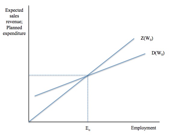
The Z-function in Figure 11.11 is drawn under the assumption that:
- The stock of capital equipment is constant.
- The money wage level is fixed.
- The productivity of labour is fixed.
A change in any of these variables would shift the function (refresh the discussion in Chapter 7 if you have forgotten how the Z-function shifts).
The other characteristic of the Z-function is that each point on Z (a given expected sales revenue) represents a particular level of income. Thus we consider at each income level, firms will estimate expected sale revenue and costs required to generate the production to meet those sales, which, in turn, defines the level of aggregate employment.
So moving up a given Z-function means the firms will be producing more output and employment more workers as income rises.
Figure 11.11 Aggregate demand (D) and Aggregate supply or proceeds (Z)

The D-function describes how much demand there will be in the economy at different (implied) income levels. We also assume that the money wage is fixed along any given D-function. Thus as employment rises, total national income rises and spending rises accordingly.
The intersection of the D- and Z-functions define the point of effective demand. In Figure 11.11, the D- and Z-functions are drawn for a given money wage level, W0, as denoted in the parenthesis.
Any point to the left of the intersection define situations where aggregate demand exceeds aggregate supply and firms would be motivated to expand production (after revising their expected sales revenue upwards in the light of inventory depletion). As a consequence, employment and income will rise until aggregate demand and aggregate supply are equal again.
Any point to the right of E0, defines a situation where aggregate supply exceeds aggregate demand and the inventory cycle will see firms reduce output, employment and income as they revise their expectations of future sales revenue downwards.
Macroeconomic equilibrium thus occurs for the current given money wage rate at E0, which determines total employment in the economy.
From our earlier discussion, the money wage impacts on both the supply and demand sides of economy. A change in the money wage changes the marginal costs at the firm level, which, in turn, impacts on the industry supply curve and thus shifts the aggregate Z-function.
At each employment level, a rise in the money wage will push the Z-function up because the firm now require more sales revenue to sustain the same employment and output levels to satisfy their profit expectations.
But, the higher money wages also means that at each employment level, incomes paid out are higher and this stimulates aggregate demand (in the first instance via higher aggregate consumption), As a consequence, the D-function shifts up when the money wage rises (and shift down in money wages are cut).
The intersection between aggregate demand (D) and aggregate supply (Z), which defines the point of effective demand, will thus be sensitive to changes in the money wage. depends on the magnitude of the money wage. This, in turn, sets the level of employment that firms will offer and the level of output and national income generated by the economy.
We can draw a family of aggregate D- and Z-functions (and points of effective demand) corresponding to different money wage levels. This, in turn, allows us to relate each money-wage level with a particular point of effective demand and aggregate employment.
Which means each point of effective demand and money wage combination constitutes a point on the macroeconomic labour demand function. The importance of the recognition is that the Classical theory of employment considered the marginal productivity function to define the macroeconomic labour demand function without reference to the goods and services market.
The approach adopted by Keynes and those who subsequently followed him, situated the derivation of the macroeconomic labour demand function in the labour market in the goods and services market – by examining how money wage movements influence the point of effective demand.
In Figure 11.11, the point E0 is thus one point on the macroeconomic labour demand function corresponding to money wage level, W0.
How we draw the family of aggregate D- and Z-functions (and resulting points of effective demand) for each money wage level depends on how changes in the money wage impacts on each function.
What happens to total employment when the money wage changes depends on how far the D- and Z- functions shift in response to the changing money wage. Three different situations can be defined:
- A money wage change shifts the D-function by less than the Z-function and thus employment falls when the money wage rises and rises when the money wage falls.
- A money wage change results in equivalent shift in the D- and Z-functions and employment does not change.
- A money wage change shifts the D-function by more than the Z-function and thus employment rises when the money wage rises and falls when the money wage falls.
In his famous 1956 article – A Macroeconomic Approach to the Theory of Wages – American economist Sidney Weintraub discussed the likely relationship between money wage changes and aggregate employment.
[REFERENCE: Weintraub, S. (1956) ‘A Macroeconomic Approach to the Theory of Wages’, The American Economic Review, 45(5), December, 835-856. The link is to JSTOR if you have library access].
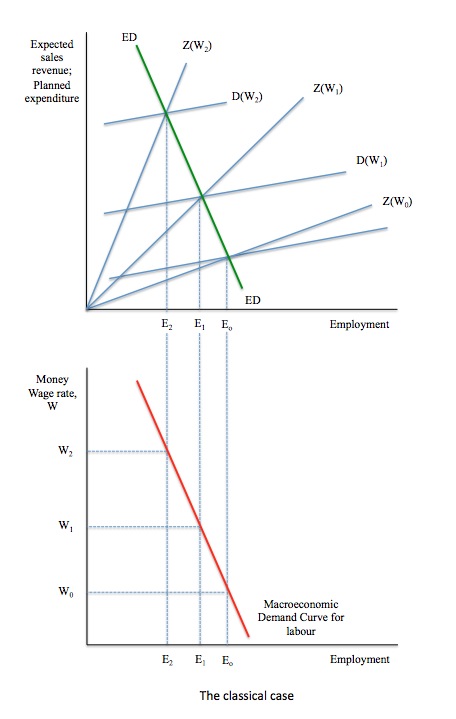
Weintraub said the first situation defined above was consistent with the traditional notion that when wages rise, employment falls. He called this the “classical”, which reflects the notion in Classical employment theory that unemployment can be eliminated by cutting money wages.
The “classical” case is shown in Figure 11.12. The upper graph shows the family of D- and Z-functions for different money wage levels, W0, W1, and W2, with W0 < W2.
The Z-function shifts upwards as the money wage rate rises by more than the D-function. The green, ED line joins the intersections of each of the points of effective demand that are established at each money wage level. These points of effective demand, in turn, determine a given employment level for each money wage level.
The lower panel in Figure 11.12 depicts the labour market, with the money wage on the vertical axis and employment on the horizontal axis. The horizontal scales on the upper and lower panels are equivalent and measure total employment.
We can thus trace the points of effective demand (where aggregate demand, D- is equal to aggregate supply, Z-) corresponding the the different money wage rates from the upper panel to the lower panel and thereby derive the macroeconomic demand for labour curve, which shows the relationship between money wages and employment.
Thus, we can derive the macroeconomic demand for labour curve by deriving all points of effective demand for all money wage levels. The lower panel thus shows that if the Z-function shifts by more than the D-function as a result of a money wage change, the resulting macroeconomic demand for labour curve will be negatively sloped.
This is what Weintraub called the “classical” case.
Figure 11.12 The Classical case

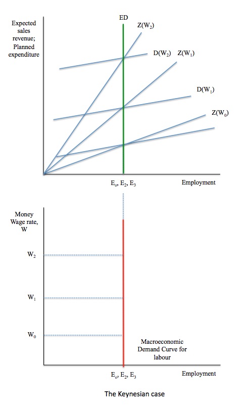
As we have seen in this discussion, Keynes attacked the Classical employment theory because he did not believe that employment was particularly sensitive to money wage movements. In terms of the three possibilities for the relative movements in the D- and Z-functions noted above, Keynes’ position corresponds to the second option – the two functions shift more or less equivalently.
Figure 11.13 captures this case, which Weintraub characterised as the “Keynesian case”. You will see that under these assumptions, the macroeconomic demand curve for labour is vertical and invariant to movements in money wages.
Figure 11.13 The Keynesian case

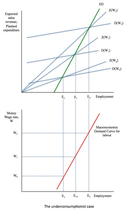
The third option – that the D-function shifts by more than the Z-function when the money wage changes, was referred to by Weintraub as the “underconsumptionist” case. The terminology was derived from a view held by some economists that money wage changes would influence consumption spending more than anything else. They believed that rising money wages would stimulate employment because the rise in consumption would push out the point of effective demand. Figure 11.14 depicts the underconsumptionist case.
Figure 11.14 The Underconsumptionist case

Weintraub (page 842) said in relation to these three cases that:
… from the standpoint of economic policy their implications are vastly different.
In other words, if, for example, the real world was more like the Keynesian or the Underconsumptionist cases, then trying to cure unemployment by cutting money wages would fail and, in the Underconsumptionist case, would be a disaster for employment.
MORE TO COME HERE
Conclusion
Tomorrow, I will complete the derivation of the macroeconomic demand for labour curve and discuss the likely impacts of money wage movements and why money wage cuts are unlikely to restore full employment.
I will draw the critique by Keynes together by way of a summary and end with some more advanced material (the part of the text that is designed for second-year macroeconomics students) about market co-ordination and the modern reinterpretation of what Keynes meant.
That is enough for today!
(c) Copyright 2013 Bill Mitchell. All Rights Reserved.
Bill, are you going to include a specific and separate section toward the end of the Keynes section dealing with contemporary critics of Keynes’ treatise, like Baylogh and Kalecki for instance, and how Keynes reacted at the time (plus perhaps your own comments)? It doesn’t have to be long and would add, I think, considerable educational value. Such historical animadversions could be placed in a box or a number of boxes as done by Misner, Thorne, and Wheeler in their monumental Gravitation. In this way such historical asides wouldn’t interrupt the flow of the main text.
May I suggest you have a brief look at Daniel Fleisch’s A Student’s Guide to Maxwell’s Equations for his innovative treatment of Maxwell’s math?
I realize that I have suggested physics books, but that in no way should be taken as a fillip to econophysics or the like, the approbation of which I consider to be a grave error on the part of many social scientists, not only economists.
I guess what I am arguing for is for a more radical pedagogical approach. So far, the book appears to me to be pedagogically conservative. Given that the content of the book is radical, should this not be accompanied by a more radical pedagogical approach, where the radical aspects of each mutually reinforce one another? The book should not just BE different; it should also LOOK different (inside, in its guts). Though not so different that students and their teachers are put off. Neither of my examples makes that mistake.
Other readers may take a different slant. This is just mine.
Bravo Bill!
So succinct that any first year economics student will be able to grasp it, unless playing rugby at their private school has bashed their brains to the point where they reject any teaching that doesn’t appear to protect their privileges.