It’s Wednesday and I just finished a ‘Conversation’ with the Economics Society of Australia, where I talked about Modern Monetary Theory (MMT) and its application to current policy issues. Some of the questions were excellent and challenging to answer, which is the best way. You can view an edited version of the discussion below and…
Unemployment and Inflation – Part 11
I am now using Friday’s blog space to provide draft versions of the Modern Monetary Theory textbook that I am writing with my colleague and friend Randy Wray. We expect to complete the text during 2013 (to be ready in draft form for second semester teaching). Comments are always welcome. Remember this is a textbook aimed at undergraduate students and so the writing will be different from my usual blog free-for-all. Note also that the text I post is just the work I am doing by way of the first draft so the material posted will not represent the complete text. Further it will change once the two of us have edited it.
This is the continuation of the Chapter on unemployment and inflation – the series so far is:
- Unemployment and inflation – Part 1
- Unemployment and inflation – Part 2
- Unemployment and inflation – Part 3
- Unemployment and inflation – Part 4
- Unemployment and inflation – Part 5
- Unemployment and Inflation – Part 6
- Unemployment and Inflation – Part 7
- Unemployment and Inflation – Part 8
- Unemployment and Inflation – Part 9
- Unemployment and Inflation – Part 10
I am now continuing the discussion of the Phillips Curve …
Chapter 12 – Unemployment and Inflation
MATERIAL HERE NOT REPEATED
[PICKING UP FROM HERE]
12.X Underemployment and the Phillips curve
As we saw in Chapter 10, underemployment has became an increasingly significant component of labour underutilisation in many nations over the last two decades. In some nations, such as Australia, the rise in underemployment has outstripped the fall in official unemployment. National statistical agencies have responded to these trends by publishing more regular updates of underemployment. They have also constructed new data series to provide broader measures of labour wastage (for example, the Australia Bureau of Statistics Broad Labour Underutilisation series, which is published on a quarterly basis).
After the major recession that beset many nations in the early 1990s, unemployment fell as growth gathered pace. At the same time, inflation also moderated and this led economists to increasingly question the practical utility of the concept of the natural rate for policy purposes, quite apart from the conceptual disagreements.
This skepticism was reinforced because various agencies produced estimates of the natural rate of unemployment that declined steadily throughout the 1990s as the unemployment rate fell. As the unemployment rate went below an existing natural rate estimate (and inflation continued to fall) new estimates of the natural rate were produced, which showed it had fallen.
This led to the obvious conclusion that the concept had no predictive capacity in relation to the relationship between movements in the unemployment rate and the inflation rate.
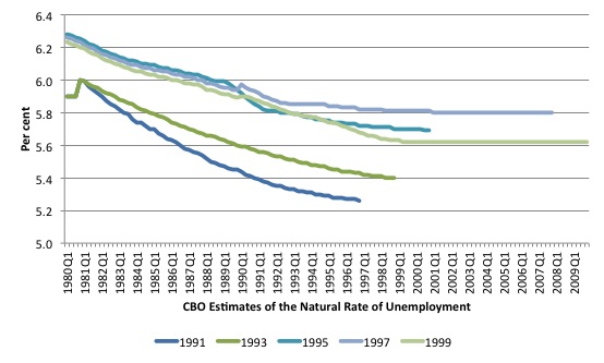
For example, in the US, the Congressional Budget Office recently (February 5, 2013) made their estimates of natural rate available – Estimates of Potential GDP and the Related Unemployment Rate, January 1991 to February 2013
The dataset provides estimates of the natural rate of unemployment in the US as computed in each January from 1991 to 1999. The estimates are back- and forward-cast, with the January 1991 estimates ending in the December-quarter 1996 and the January 1999 estimates ending in the fourth-quarter 2009
Figure 12.13 shows the various estimates (in two-yearly intervals) for the period 1980Q1 to the end of each estimated sample. There are two characteristics of the time series. First, the CBO arbitrarily pushed the estimated natural rate of unemployment between 1991 and 1995. Second, for each of the time-series estimates the natural rate was falling, particularly in the 1990s.
Figure 12.13 Congressional Budget Office estimates of the Natural Rate of Unemployment

Source: CBO, Estimates of Potential GDP and the Related Unemployment Rate, January 1991 to February 2013, February 5, 2013.
While there are various explanations that have been offered to rationalise the way the estimated natural rates of unemployment fell over the 1990s (for example, demographic changes in the labour market with youth falling in proportion), one plausible explanation is that there is no separate informational content in these estimates and they just reflect in some lagged fashion the dynamics of the unemployment rate – that is, the hysteresis hypothesis.
The question then arises as to why the unemployment rate and the inflation rate both fell in many nations during the 1990s. What does this mean for the Phillips curve?
To understand this more fully, economists started to focus on the concept of the excess supply of labour, which is a key variable constraining wage and price changes in the Phillips curve framework.
The standard Phillips curve approach predicts a statistically significant, negative coefficient on the official unemployment rate (a proxy for excess demand). However, the hysteresis model suggests that state dependence is positively related to unemployment duration and at some point the long-term unemployed cease to exert any threat to those currently employed.
Consequently, they do not discipline the wage demands of those in work and do not influence inflation. The hidden unemployed are even more distant from the wage setting process. So we might expect that the short-term unemployment is a better excess demand proxy in the inflation adjustment function.
While the short-term unemployed may be proximate enough to the wage setting process to influence price movements, there is another significant and even more proximate source of surplus labour available to employees to condition wage bargaining – the underemployed.
The underemployed represent an untapped pool of potential working hours that can be clearly redistributed among a smaller pool of persons in a relatively costless fashion if employers wish.
It is thus reasonable to hypothesise that the underemployed pose a viable threat to those in full-time work who might be better placed to set the wage norms in the economy.
This argument is consistent with research in the institutionalist literature that shows that wage determination is dominated by insiders (the employed) who set up barriers to isolate themselves from the threat of unemployment. Phillips curve studies have found that within-firm excess demand for labour variables (like the rate of capacity utilisation or rate of overtime) to be more significant in disciplining the wage determination process than external excess demand proxies such as the unemployment rate.
It is plausible that while the short-term unemployed may still pose a more latent threat than the long-term unemployed, the underemployed are also likely to be considered an effective surplus labour pool. In that case we might expect downward pressure on price inflation to emerge from both sources of excess labour.
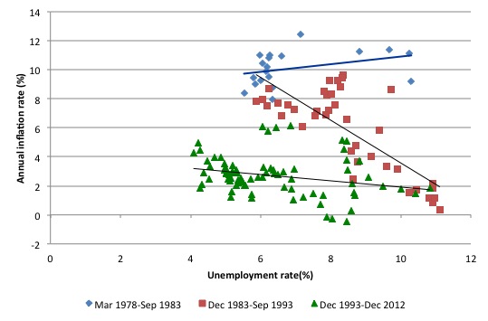
Figure 12.14 shows the relationship between the unemployment rate and inflation in Australia between 1978 and 2012. The sample is split into three sub-samples. The first from March 1978 to September 1983 is defined by the starting point of the most recent consistent Labour Force data (February 1978) and the peak unemployment rate from the 1982 recession (September 1983).
The second period December 1983 to September 1993 depicts the recovery phase in the 1980s and then the period to the unemployment peak that followed the 1991 recession. The final period goes from December 1993 to December 2012.
The solid lines are simple linear trend regressions.
Figure 12.14 Inflation and unemployment, Australia, 1978-2013

Source: Australian Bureau of Statistics, Consumer Price Index and Labour Force.
The relationship between the annual inflation rate and the unemployment rate clearly shifted after the 1991 recession. The graph shows three particular points (September 1995, September 1996, and September 1997) as the Phillips curve was flattening and moving inwards. So over these years, the unemployment rate was stuck due to a lack of aggregate demand growth but the inflation rate was falling.
This has been explained, in part, by the fall in inflationary expectations. The 1991 recession was particularly severe and led to a sharp drop in the annual inflation rate and with it a decline in survey-based inflationary expectations.
The other major labour market development that arose during the 1991 recession was the sharp increase and then persistence of high underemployment as firms shed full-time jobs, and, as the recovery got underway, began to replace the full-time jobs that were shed with part-time opportunities. Even though employment growth gathered pace in the late 1990s, a majority of those jobs in Australia were part-time. Further, the part-time jobs were increasingly of a casual nature.
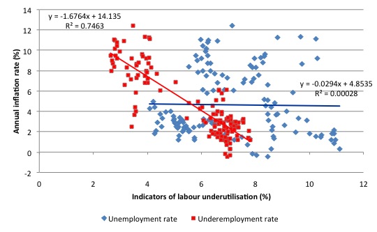
Figure 12.15 shows the relationship between unemployment and inflation from 1978 to 2012. It also shows the relationship between the underemployment estimates provided by the Australian Bureau of Statistics and annual inflation for the same period.
The equations shown are the simple regressions depicted graphically by the solid lines. The graph suggests the negative relationship between inflation and underemployment is stronger than the relationship between inflation and unemployment. More detailed econometric analysis confirms this to be the case.
Figure 12.15 Inflation and unemployment and underemployment, Australia, 1978-2013

Source: Australian Bureau of Statistics, Consumer Price Index and Labour Force.
The inclusion of underemployment in the Phillips curve specification helps explain why low rates of unemployment have not been inflationary in the period leading up to the Global Financial Crisis. It suggests that shifts in the way the labour market operates – with more casualised work and underemployment – have been significant in explaining the impact of the labour market on wage inflation and general price level inflation.
Conclusion
Next week I will move into a broader discussion of conflict theories of inflation and supply-side (raw material) shocks. I will propose this is a general Modern Monetary Theory framework for understanding inflation.
Then we move onto how the Phillips curve can be rendered irrelevant through employment buffers.
Saturday Quiz
The Saturday Quiz will be back again tomorrow. It will be of an appropriate order of difficulty (-:
That is enough for today!
(c) Copyright 2013 Bill Mitchell. All Rights Reserved.
Letter in Toronto Star
http://www.thestar.com/opinion/letters_to_the_editors/2013/03/25/austerity_budget_means_more_of_the_same.html
Re: Flaherty says balanced budget prepares country for another crisis, March 22
Sovereign countries like Canada and the U.S. cannot run out of their own money. U.S. Federal Reserve Governor Ben Bernanke has stated, “the U.S. government has a technology, called a printing press (or, today, its electronic equivalent), that allows it to produce as many U.S. dollars as it wishes at essentially no cost.”
Those who say federal coffers are bare or ask where federal money will come from are simply misinformed. Greece and Cyprus may have surrendered their monetary sovereignty to a foreign central bank, but Canada has not.
The rational debate is over the effects of an injection of fiat money into the economy. A reminder that during World War II, our budget deficit rose above 42 per cent of GDP, and our debt-to-GDP ratio was over three times what it is today. The results were a rapid increase in production from the Depression years, unemployment was driven down to 1 per cent, and a military victory was followed by years of prosperity, all with limited inflation.
Finance Minister Jim Flaherty says his proposed balanced budget prepares our country for another potential crisis. However, the main effect of failing to stimulate the economy now will be to keep over a million Canadians unemployed and to keep many families heavily indebted. This will not protect us from a future crisis; in fact, it will more likely help precipitate one.
Larry Kazdan, Vancouver
________________________________________________________________________________
P.S. A footnote link to Billy Blog (Bernanke quote) was included in the original letter to editor. Toronto Star is Canada’s largest paper by circulation.
Perceptions on affordability
No single dominant policy question these days affect our daily lives more than diverging perceptions of affordability of government spending. Some opinnion that government has very limited room to increase spending before affordability becames an issue. Prevalence of this opinnon reflects a failure of our education system to give accurate picture of government spending procedures to hordes of otherwise well-educated commentators and policy experts. etc.
Re the divergent opinions on govt spending, it seems to me that the fundamental problem is that the field of economics is unable to agree on the appropriate evidential context needed to answer such questions or it deems evidence irrelevant or both.
It’s more fundamental than that IMHO.
In situations of fundamental uncertainty, the only way you can see if something works is to try it and see and if it doesn’t back out and try something else.
And of course the reason for that is that ‘evidence’ is only ever circumstantial until you try what you want to try. And that leads to the usual problems of bias, curve fitting and seeing Teddy Bears in the data.
In IT we call it ‘analysis paralysis’, and those who prefer the status quo use Fear, Uncertainty and Doubt (FUD) to try and prevent the change. The job of the change agent is to overcome those techniques and demonstrates that the rewards of a successful change outweigh the risks.
Sell the benefits.
Economists will say that their theories are just ‘opinions’. That’s what the credit rating agencies used in their defence.
Everyone can have their own opinions, right? There is no need for opinions to be factually accurate.
Role of the education system on the other hand is to inform people not mislead them.
Is it possible that household debt is another factor to consider? Steve R Waldman has written about how household indebtedness was used in “the great moderation” to ensure CPI inflation and wages did’t increase without actually making people lose jobs so much. If people are in debt they daren’t agitate for higher wages. Also the debt burden means that interest rates quickly reduce household spending capacity as soon as inflation threatens. When interest rates drop, more credit is made available and the spending on credit makes low wages seem less unfair. It came to a head once household debt got maxed out and interest rates had progressively dropped to zero. That has left us where we are now.
As an aside, as a rhetorical way of exposing the injustice of some economic arguments, it could be pointed out that the ultimate way to get the NAIRU down to zero would be to reinstate the system of fines for vagrancy and indentured labor as a way to pay off the fine by a lifetime of work in service of whoever offers to pay the fine. It worked in the post-slavery American South.