It’s Wednesday and I just finished a ‘Conversation’ with the Economics Society of Australia, where I talked about Modern Monetary Theory (MMT) and its application to current policy issues. Some of the questions were excellent and challenging to answer, which is the best way. You can view an edited version of the discussion below and…
Analytical appendix for NIPA Chapter 3 – Part 3
I am now using Friday’s blog space to provide draft versions of the Modern Monetary Theory textbook that I am writing with my colleague and friend Randy Wray. We expect to publish the text sometime in 2013. Our (very incomplete) textbook homepage – Modern Monetary Theory and Practice – has draft chapters and contents etc in varying states of completion. Comments are always welcome. Note also that the text I post here is not intended to be a blog-style narrative but constitutes the drafting work I am doing – that is, the material posted will not represent the complete text. Further it will change as the drafting process evolves.
The Table of Contents for the first draft, which is nearly completed, currently lists Chapter 3 as National Income Accounting, with a section 3.7 Using the NIPA Framework to Model the Macro Economy. The status of this section might change but the content aims to present some analytical terminology that is used in the specification of macroeconomic models which the student encounters throughout the textbook.
The section (or subsection) will cover basic algebra, manipulation of equations, solving simple linear models, consideration of graphs, and some essential tools that help an applied macroeconomist assess data trends etc.
Today, I am adding to the material already developed which is currently available as Chapter 3 Draft, Section 3.8.
The snippets I develop here will be integrated into the draft for further assessment. The ambiguity of the numbering reflects the transient status of these sections.
The other parts of this section of the text:
[CONTINUING FROM HERE]
Index numbers
Index numbers allow comparisons between two or more variables over time. This can be especially helpful if the units of the underlying variables or their levels differ and make it difficult to easily relate their movements.
The creation of an index number requires a starting point (the base period or value) which is usually set at 100. Each subsequent observation is then expressed as a percentage of the base year. An index number is unit free.
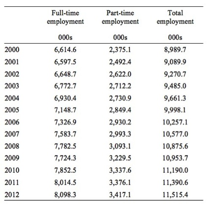
For example, consider the data in Table A1, which shows full-time, part-time and total employment for Australia from 2000 to 2012. The data is reported in units of thousands.
Visual inspection of the data can provide information as to the evolution of employment over this time period in Australia.
But what if we wanted to know whether full-time employment had grown faster or slower than part-time employment since 2000? This is where index numbers are useful.
Table A1 Employment in Australia, 2000-12, 000s
Source: Australian Bureau of Statistics, Labour Force – http://www.abs.gov.au/AUSSTATS/abs@.nsf/mf/6202.0
To convert this data into index numbers we define the base as the year 2000 and call that value 100. In computational terms, for full-time employment, we would calculate 100*(6,614.6/6,614.6) = 100 and so on for the other variables of interest.
The index number full-time employment for 2001 would thus be 100*(6,597.5/6,614.6) = 99.7 and so on.
Table A2 shows the index numbers corresponding to the three employment time series. Note that while the raw employment data is expressed in units of thousands, the index numbers are unit free. It is common practice to define the base period which in this case is 2000=100.
Table A2 Employment indices for Australia, 2000-12
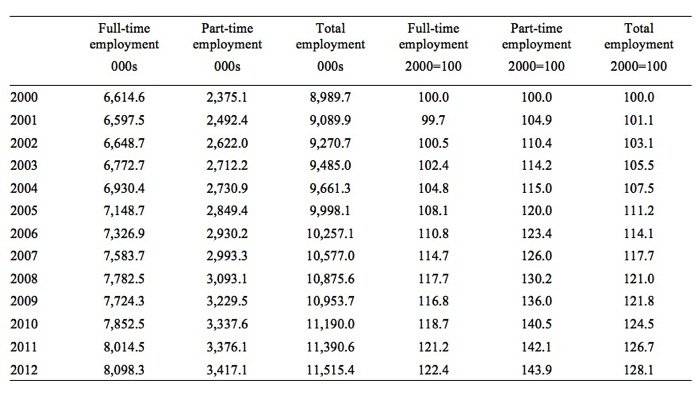
We can see that the index number for full-time employment rose from 100 in 2000 to 122.4 in 2012, a 22.4 per cent increase, while the part-time employment index number rose from 100 in 2000 to 143.9 in 2012, a 43.9 per cent rise, almost twice as large an increase as full-time employment.
Note that for any pair of index number observations we can also compute percentage changes. For example, what was the growth of full-time employment in 2008 and 2009?
We know that full-time employment was 7,782.5 in 2008 and had fallen to 7,724.3 in 2009. We could calculate a simple percentage 100*(7,724.3 – 7,782.5)/7,724.3 = -0.75 per cent.
We could find the same result using the index numbers 117.7 in 2008 and 116.8 in 2009 and computing 100*(116.8/117.7) – 100.
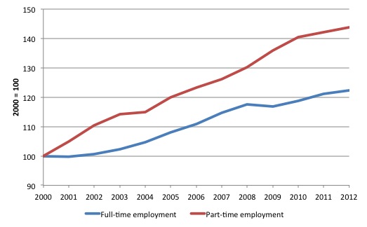
It is also useful to graph index numbers if we are interested in a visual comparison of the behaviour of different variables.
For example, the visualisation easily allows one to see that in 2008, when the financial crisis emerged, full-time employment in Australia contracted while part-time employment accelerated. This observation would motivate a researcher to investigate the labour market processes that underpinned this outcome.
Figure A5 Employment index numbers, Australia, 2000-2012, 2000=100
Index numbers also allow us to compare the evolution of two or more different variables over time when the underlying units of measurement of each variable are different.
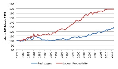
For example, for decades real wages in most nations grew in line with labour productivity. The latter created the space for the former to growth without invoking inflationary pressures. So economists are often interested in examining the relationship between the two variables over time.
Figure A6 shows the relationship between real wages and productivity growth in Australia from 1978 to 2012 in index number form where the base period is March 1978. The underlying data is quarterly.
Productivity is measured in terms of units of real GDP per hour worked while real wages are computed as the nominal wage series ($ per hour) deflated by the consumer price index.
By converting the different series in common index numbers we are readily able to see the comparative behaviour of these related time series.
Figure A5 Real wages and productivity, 1978- 2012, March-quarter 1978=100
Source: Mitchell (2013).
Price index numbers
Price indexes are used to provide a measure of the general movement in prices.
There are many different examples, such as, wholesale and retail price indexes. The Consumer Price Index (CPI) is a well-known and often-quoted example of an index number.
It is calculated by assuming a given basket of goods and services are representative of the purchases made by a typical household. The index then traces the change in value or cost of that basket over time and so provides a measure of the change in the cost-of-living.
The measure is usually expressed for a specific spatial area such as a capital city or a weighted-average of all capital cities in a nation.
The items included in the Australian CPI published by the Australian Bureau of Statistics are shown in Table A2. Within each major group there are many items included.
Table A2 Items in Australian CPI, September 2013
All groups CPI
Food and non-alcoholic beverages
Alcohol and tobacco
Clothing and footwear
Housing
Furnishings, household equipment and services
Health
Transport
Communication
Recreation and culture
Education
Insurance and financial services
Source: Australian Bureau of Statistics, Consumer Price Index, http://www.abs.gov.au/AUSSTATS/abs@.nsf/mf/6401.0
If the prices of all the items in the basket moved proportionately between periods then the movement in the general prices would be easy to calculate.
But, in reality, the individual components generally change at different rates, that is, the relative prices are also changing. The statistician thus needs a single summary measure to determine whether the basket overall is rising in cost or not. That is the role that the price index plays. It is a weighted-average of the price movements in the given basket relative to some base period.
In compiling a summary measure such as the CPI the statistician has various options. Two broad options are whether to use base-weighting or current-weighting to compile the index.
A base-weighted index examines the shifts in prices of the basket of goods and services using the base-period quantities purchased and is referred to as a Laspeyres index after the German economist who first compiled such measures.
The base-weighted index allows us to see how much a basket that consumers bought in the base period would cost in the current period.
A current-weighted index uses the current quantity purchased of each good and service in the basket as the weight to compile the average measure. This is commonly called a Paasche index after the German statistician who derived this measure.
The current-weighted index allows us to see how much a basket that consumers buy in the current period would have cost in the base period.
Both measures provide different ways of estimating the change in the cost of the basket of goods and services over time. However, statisticians tend to favour the use of the Laspeyres index to calculate the CPI because it requires less information to be available. It only requires the current prices of the items in the basket to be known.
This allows for a more timely publication of the CPI, which is a central policy variable used by central bankers and treasuries in formulating monetary and fiscal policy, not too mention, its use in labour and other contracts.
To simplify our analysis, imagine a basket of goods and services comprises two items (Bread and Cheese). Yes, the obvious question, don’t these people wear clothes?
Table A3 shows the hypothetical data we will be working with to illustrate the construction of the price index.
Table A3 Hypothetical data for basket of goods and services
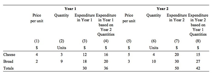
In Year 1, the price per unit of Cheese is $4 and 3 units are consumed overall. So total expenditure on Cheese in Year 1 is $12. The price of a loaf of Bread is $2 and 9 units are consumed in Year 1, making total expenditure on Bread $18. Overall, the basket of goods costs $30 in Year 1 (Column 3).
In Year 2, Cheese rises to $5 per unit and 4 units are consumed whereas Bread rises to $3 per loaf and 10 units are consumed. Overall, the basket of goods in Year 2 now costs $50 (Column 7).
Note that if we wanted to know what the Year 1 purchase quantities would cost in Year 2, Column (8) provides that answer, $42.
We calculated that using the following formula:
Cheese $5 x 3 = $15
Bread $3 x 9 = $27
Total = $42
The 3 and the 9 are the quantities of each good purchased in Year 1. Conversely, Column (7) shows the expenditure in Year 2 based on Year 2 prices and Year 2 purchases.
Similarly, if we wanted to know what the basket would cost in Year 1 based on Year 1 prices and Year 2 purchases we would look to Column (4).
What would be the price index numbers in this example?
Base-weighted CPI
Using base-weights (Year 1 quantities), the index in Year 1 would be:
CPIYear 1 = 100 x Total Expenditure in Year 1 (Column 3) divided by Total Expenditure in Year 1 (Column 3)
CPIYear 1 = (100 x $30)/$30 = 100
In Year 2, the index would be (using Year 1 weights):
CPIYear 2 = 100 x Total Expenditure in Year 2 (Column 8) divided by Total Expenditure in Year 1 (Column 3)
CPIYear 2 = (100 x $42)/$30 = 140
This would suggest that the percentage change in prices was 40 per cent between Year 1 and Year 2.
This is not the rate of inflation because we would need a further data point before we could conclude there was an continuing change in the price level.
Current-weighted CPI
Using current-weights (Year 2 quantities), the index in Year 1 would be:
CPIYear 1 = 100 x Total Expenditure in Year 1 (Column 4) divided by Total Expenditure in Year 1 (Column 4)
CPIYear 1 = (100 x $36)/$36 = 100
In Year 2, the index would be (using Year 1 weights):
CPIYear 2 = 100 x Total Expenditure in Year 2 (Column 7) divided by Total Expenditure in Year 1 (Column 4)
CPIYear 2 = (100 x $50)/$36 = 138.9
This would suggest that the percentage change in prices was 38.9 per cent between Year 1 and Year 2.
You will appreciate that the current-weighted index takes into account changes in both prices and quantities purchased, whereas the base-weighted approach considers price changes only and ignores the fact that people will change their expenditure patterns over time as relative prices change.
In practice, statisticians periodically revise the weights in the basket of goods and services in line with other information they collect with respect to household expenditure patterns. They then have complex methods to splice the new and the old indexes together.
Textbook policy regarding formalism
We recognise that different students have different ways in which they learn and accumulate knowledge. Some prefer the mathematical approach while others prefer the graphical approach. Others still learn better through reading the written word, even though that form of communication is prone to interpretative issues.
In that regard, all the essential material in the text will be presented in all three ways (sometimes the mathematics will appear in the Annexe of the relevant chapter sometimes within the main body of the text.
We always aim to promote understanding and believe that a student is entitled to learn in the way that best suits their own proclivities.
However, it is also the case that professional economists use a variety of methods including numerical, graphical, algebraic and narrative in their work and we believe it is important to expose students to the broad range of methods deployed in the real world.
Conclusion
I am now going back through the first draft and editing, adding and refining sections.
Saturday Quiz
The Saturday Quiz will be back again tomorrow. It will be of an appropriate order of difficulty (-:
That is enough for today!
(c) Copyright 2013 Bill Mitchell. All Rights Reserved.
Prof, I’m thinking that business spending (I) in the US is a function of the stock market because entrepreneurs and investors invest in private companies hoping to make a fortune after taking them public. Merry Christmas!