It’s Wednesday and I just finished a ‘Conversation’ with the Economics Society of Australia, where I talked about Modern Monetary Theory (MMT) and its application to current policy issues. Some of the questions were excellent and challenging to answer, which is the best way. You can view an edited version of the discussion below and…
Growth and Inequality – Part 1
I am now using Friday’s blog space to provide draft versions of the Modern Monetary Theory textbook that I am writing with my colleague and friend Randy Wray. We expect to publish the text sometime around mid-2014. Our (very incomplete) textbook homepage – Modern Monetary Theory and Practice – has draft chapters and contents etc in varying states of completion. Comments are always welcome. Note also that the text I post here is not intended to be a blog-style narrative but constitutes the drafting work I am doing – that is, the material posted will not represent the complete text. Further it will change as the drafting process evolves.
Chapter X Growth and Inequality
X.1 Overview
Throughout this textbook we have been examining what determines fluctuations in the trade cycle. This has typically been referred to as short-run analysis, because it assumes that the stock of productive capital available (machinery, equipments, skills and experience, etc) are fixed over the period the analysis is being conducted.
We have also noted that contemporary issues relating to the ageing society and reducing poverty rates in nations requires a consideration of what economists term the long-run. In this regard, we focus on what determines productivity and productivity growth.
Productivity growth, which allows real income to grow, is the single most important determinant of our material standard of living and the trading standings between nations.
When we considered the determinant of aggregate supply and employment we were content to define productivity as output per unit of input.
We thus calculated labour productivity as the total value of real output divided by total employment or total hours worked. So if a firm produced 1000 units of output each day and employed 100 workers in the process, then the labour productivity of that plant would be 10.
There are many conceptual issues involved in measuring labour productivity. For example, it is rarely the case that we can isolate productive inputs. Further, how do we account for different labour skills that are deployed to produce a given volume of output?
Economists also compute measures of total factor productivity which attempts to include the contributions to final output of all the inputs used – capital, labour, organisation, etc.
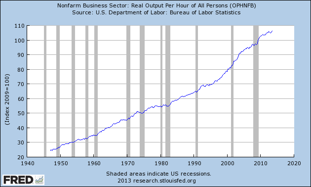
Figure X.1 shows real output per hour worked index for the US nonfarm business sector (2009=100). The grey bars are the US recession periods as specified by the National Bureau of Economic Research.
There are two points to note. First, productivity is a cyclical variable, tending to decline during a recession and pick up at the end of the recession. We have discussed this phenomena in Chapter 13.
To refresh your memory, when firms face declining orders, they reduce output at a slower rate than they reduce their workforce. firms tend to hoard certain categories of labour during an downturn in the economic cycle. For example, firms are reluctant to sack skilled labour because it is expensive to recruit and train. Further, maintenance of operations requires a certain complement of overhead labour, for example, front-desk staff, telephonists etc.
Firms also will turn machines off or run their capital at slower speeds as they adjust their output volumes down to meet the declining sales volume.
Thus productivity declines during a downturn because less output is being produced for a given quantity of inputs.
In the recovery, as sales pick up, output rises and the hoarded labour works more intensively and machinery is brought back into higher rates of utilisation. As a result productivity rises.
Second, productivity grows over time at various rates. We call this the long-run or secular trend in productivity.
For the US, the 1980s were a period of slower productivity growth relative to earlier and later periods. In this chapter we will consider what determines long-run productivity growth.
Figure X.1 Nonfarm Business Sector: Real Output Per Hour of All Persons, US, 1940-2013, 2009=100

Source: U.S. Department of Labor: Bureau of Labor Statistics, Productivity and Costs.
The US Bureau of Labor Statistics (BLS) provides an excellent source of data that permits international labour comparisons – http://www.bls.gov/fls/
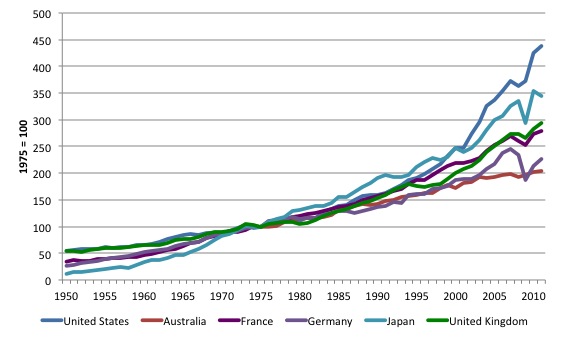
Figure X.2 compares the evolution of output per employed person in manufacturing for selected nations from 1950 to 2011 (1875 = 100).
The common base year allows us to compare relative growth rates in productivity across nations. In the period since 1975, Japan was the leading nation as its pace of industrialisation expanded but by 1999, the US had overtaken Japan, which still remained ahead of the other nations shown.
Australia and Germany have been relatively low productivity nations with the UK and France tracking each other closely.
Once again you can see the marked cyclical behaviour of productivity during global financial crisis (2009) where productivity fell sharply in most nations.
Figure X.2 Output per employed person in manufacturing in selected nations, 1950-2013, 1975=100

Source: U.S. Department of Labor: Bureau of Labor Statistics, International Labor Statistics.
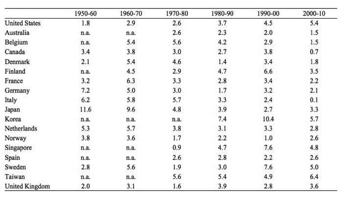
Table X.1 shows annual percentage growth in Output per employed person in manufacturing in selected nations from 1950-51 to 2010-11.
The data provides a rich source of information on the shifting world patterns in manufacturing over time. For example, in the immediate Post World War II period, the reconstruction of Japan meant it achieved outstanding productivity growth relative to the other nations. The war-torn European nations (Germany, Italy, Netherlands) also enjoyed strong productivity growth.
More recently, the newly industrialising nations such as Korea and Singapore have enjoyed strong growth as the more mature industrial nations have witnessed slowing productivity growth.
To help you understand the implications of the productivity growth variations consider Australia, which in the decade to 2000 grew on average at 2 per cent per annum but slowed to 1.5 per cent per annum in the decade 2000-10.
Using compounding formula (the well-known Rule of 72 – see box), we know that if productivity growth is 2 per cent, then real income will double every 36 years.
If productivity growth drops to 1.5 per cent, then real income will double every 48 years. In the case of the US, where productivity growth was averaging 5.4 per cent per annum between 2000-10, real income will double each 13 odd years. Of-course, before we can conclude what this means for the average citizen we also would need to know about the distribution of income. The US has rising income inquality and is overall less equal than Australia, so the advances in material standards of living provided for by productivity growth are less evenly shared in the US than, say, in Australia.
Table X.1 Output per employed person in manufacturing in selected nations, 1950-2013, 1975=100

Source: U.S. Department of Labor: Bureau of Labor Statistics, International Labor Statistics.
X.2 Keynesian growth theories – Harrod-Domar
An early growth theory came from Roy Harrod in 1939 when he attempted to provide a long-run reconstruction of Keynes’ General Theory. Eight years later, Evsey Domar introduced a model of long-run growth, which added to the approach taken by Harrod. It is conventional to refer to this work as the Harrod-Domar growth model.
There are three components to their model:
1. The warranted rate of growth, which is the rate of growth that maintains full utilisation of capital.
2. The natural rate of growth, which is the rate of growth that ensures that all workers that desire work can find employment. Equilibrium occurs when the warranted rate of growth equals the natural rate of growth.
3. The razor’s edge or instability of growth, where the two rates of growth which define a full employment equilibrium are prone to deviate and cause crisis.
To see the derivation of the Harrod-Domar model we assume a very simple model of income determination:
(X.1) Yt = Ct + It
where Yt is total output/income in period t, Ct is total consumption in period t, and It is total investment in period t.
We are assuming a closed economy for simplicity.
Income can be either consumed or saved and St = sYt, where s is the marginal propensity to save (which is 1 – the marginal propensity to consume).
Thus:
(X.2) Yt = Ct + It = Ct + St
In equilibrium:
(X.3) St = It
Capital is accumulated over time according to the following expression:
(X.4) Kt+1 = It + Kt(1 – δ)
where K is the capital stock, and δ is the rate of depreciation of the existing capital stock (Kt). In other words, the capital stock increases as a result of the flow of investment in the current period taking into account the depreciation of existing capital.
From, Equation (X.3), we can re-write the capital accumulation relationship as:
(X.5) Kt+1 = sYt + Kt(1 – δ)
If we assume there is no depreciation (δ = 0) then (X.5) simplifies to:
(X.6) Kt+1 = sYt + Kt
Noting that ΘKt+1 – ΘKt = ΔK, then:
(X.7) ΔKt = sYt
Warranted rate of growth
The warranted rate of growth ensures that all available capital is fully employed.
We define a fixed output-capital ratio which is an indicator of the productivity of capital:
(X.8) Θ = Yt/Kt
The magnitude of Θ determines how much capital is required per unit of output. High values of Θ means that a nation will require large capital stocks to produce and vice versa. For now, we will abstract from issues such as quality of capital and how we might value the heterogenous items (machines, equipment etc) that are aggregated in a single measure of a nation’s capital stock.
Note that:
(X.8) Yt = ΘKt
If Θ is fixed, then Equation (X.7) means that to increase output, more capital has to be added in proportions dictated by Θ
Thus:
(X.9) ΔYt = ΘΔKt
If we substitute Equation (X.7) into (X.9) we get:
(X.10) ΔYt = ΘsYt
If we divide both sides by Yt, Equation (X.10) becomes a growth relationship:
(X.11) g = Θs
We drop the subscripts to simplify and note that g is the warranted rate of growth in output, which given the fixed output-capital ratio will ensure the current capital stock is fully utilised.
Natural rate of growth
NEXT WEEK AND ANALYSIS OF INSTABILITY
References
Domar, E. (1947) ‘Expansion and Employment’, American Economic Review, 37, 34-55.
Harrod, R. (1939) ‘An Essay in Dynamic Theory’, Economic Journal, 49, 14-33.
Conclusion
CONTINUING NEXT FRIDAY.
Saturday Quiz
The Saturday Quiz will be back again tomorrow. It will be of an appropriate order of difficulty (-:
That is enough for today!
(c) Copyright 2013 Bill Mitchell. All Rights Reserved.
“In the downturn, as sales pick up, output rises ”
During the recovery?
Dear Neil Wilson
Thanks for the typo spotting.
best wishes
bill
Bill –
If it’s typos you’re after, you’ve got the declining salves volume and from 1950 to 2011 (1875 = 100).
But I think a bigger problem is the labelling of figure X.2, as it really shows output growth rather than output, and it doesn’t explain how you’re addressing the problem that Germany was two nations for most of the time graphed.
(X.6) Kt+1 = sYt + Kt
Noting that ΘKt+1 – ΘKt+1 = ΔK, then:
(X.7) ΔKt = sYt
shouldn’t that be
ΘKt+1 – ΘKt = ΔK
?
Isn’t there a bit of a confounding issue though when interpreting “output per employed person in manufacturing”? If a country becomes say financialized (or messed up in some other way) and almost all manufacturers go bust, then perversely that could boost “output per employed person in manufacturing”. Imagine a country starts off with say 10000 people employed in ” fancy manufacturing” making F1 cars and satellites and those workers have very high output AND the country also has world class mass market car manufacturers and textile industry etc that employ 10000000 people at world class output for those industries but nevertheless considerably lower output than for the “fancy manufacturing”. If all of that is laid waste and we are just left with the fancy manufacturing with everyone else on the dole or working for a pittance in call centres, then we will get a big boost to “output per employed person in manufacturing” won’t we.
Is this effect what makes Germany seem to lag the UK – in the UK we only have fancy manufacturing remaining?
Dear hamstray (2013/12/29 at 3:54)
Thanks for the typo correction.
Fixed now.
best wishes
bill
Professor Bill
Best wishes for the Holiday season !
I look forward to release of the MMT text. There is much about MMT that I find attractive. But I have some serious concerns as well but these may stem from ignorance. Trying to develop a complete understanding of MMT by reading blogs is fraught with peril.
(X.6) Kt+1 = sYt + Kt
Noting that ΘKt+1 – ΘKt = ΔK, then:
(X.7) ΔKt = sYt
Implies theta =1
Tanks for a great website
(X.1) Yt = Ct + It
where Yt is total output/income in period t, Ct is total consumption in period t, and It is total investment in period t.
We are assuming a closed economy for simplicity.
Income can be either consumed or saved and St = sYt, where s is the marginal propensity to save (which is 1 – the marginal propensity to consume).
Thus:
(X.2) Yt = Ct + It = Ct + St
In equilibrium:
(X.3) St = It
Surely going from x1 to x2 requires It =St
Also, if equilibrium is defined by Ct= 0 which x2 and x3 implies, Then Ct is a rate of change in consumtion. Is that so?
Best regards
Jon
Dear Jon (at 2014/01/18 at 8:26)
You note that if Yt = Ct + It = Ct + St then S=I. Always. But that doesn’t necessarily mean equilibrium as you infer. For equilibrium, planned saving has to equal planned investment. That is, the firms have to have produced the right combination of goods (consumption and investment goods) in advance which mesh with the plans of the households. Actual saving and actual investment, in this simple model will always be equal by definition of the accounts. But the plans might not mesh – why? If firms overestimate consumption, they will produce more goods and services than they actually end up selling and will accumulate inventories.
These stockpiles of unsold goods and services are called Unintended Investment (inventories are counted as investment in the national accounts). So total investment is split between planned and unplanned. Which means S=I may not be an equilibrium state.
Then you say in equilibrium C=0. Why? Even in the simple equation you list Ct + It = Ct + St, C could be 80, S = 20, I = 20 and the equation would hold. Ct is not the growth in consumption it is the flow of consumption spending. The difference between that and disposable income is saving.
I hope that helps.
best wishes
bill