It's Wednesday and I discuss a number of topics today. First, the 'million simulations' that…
US labour market weakening
The Federal Reserve Bank of America has been publishing a new indicator – the Labor Market Conditions Index (LMCI) – which is derived from a statistical analysis of 19 individual labour market measures since October 2014. It is now being watched by those who want to be the first to predict a rise in US official interest rates. If the latest data from the LMCI is a guide to potential interest rate movements then they won’t be rising any time soon. I updated my gross flows database today and also the job openings and quits database. The gross flows analysis suggests that while there has been improvement in the US labour market in the last year, in recent months that improvement is slowing.
The statistical construction of the LMCI would be of interest to some readers but not many. The index is derived from a “dynamic factor model”, which extracts common variations from the individual indicators used as the raw data – which include measures of Unemployment and underemployment, employment, working hours, wage movements, vacancy rates, hiring, layoffs, and quits and measures of consumer and business confidence.
Dynamic Factor Models are increasingly being used in macroeconomics where economists have a huge number of variables of interest but the number of observations for each of the variables (time series) are fairly short. By combining many data series the sample becomes large and the so-called degrees of freedom problem that plagues regression-based time series modelling is overcome.
The idea is that over time a few unobserved dynamic factors can explain a high proportion of the co-movement in a number of labour market variables. The statistician estimates these factors (using a range of tools such as the Principal Components estimator) and then using the components as weights in an index (roughly speaking).
The 19 individual labor market measures do not impact equally on the movement of the LMCI. The “most strongly related” are the unemployment rate, private payroll employment, the “composite help-wanted index, the insured unemployment rate, the quit rate, and persons working part-time for economic reasons”.
The data is detrended before use so that the ‘level’ of the index has “no obvious economically-meaningful interpretation”. Accordingly, the “ndex captures common movements only among the cyclical deviations of the indicators from their estimated trends, neglecting any common movements in those trends.”
So only changes in the index are worth studying. The resulting short-run changes in the LMCI are “assumed to summarize overall labor market conditions”.
My own research centre has created two indexes – the CofFEE Employment Vulnerability Index – and an unpublished (as yet) Economic Prosperity Index – which use this statistical methodology.
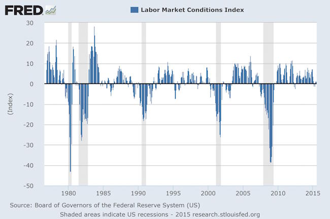
The following graph (constructed at FRED) shows the full span of the LMCI from August 1976 to July 2015. The shaded areas show official US recessions.
The second graph just zooms in to the period January 2007 to July 2015 and gives you a better impression of the monthly changes.
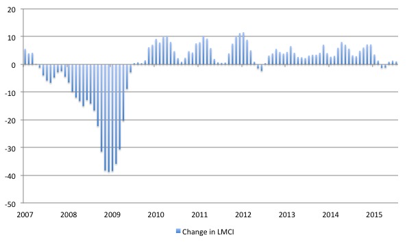
The conclusion is that the current labour market is relatively weak (compared to last year). To understand that we note that while unemployment is now lower than last year, the rate of hiring is also slower and the way these factors combine in the index leads to an overall assessment that the labour market is in decline.
I also thought I would update the Transition Probabilities that can be derived from the Gross Flows labour market data.
To fully understand the way gross flows are assembled and the transition probabilities calculated you might like to read these blogs – What can the gross flows tell us? and More calls for job creation – but then. For earlier US analysis see this blog – Jobs are needed in the US but that would require leadership
The data is available from the – US Bureau of Labor Statistics.
Gross flows analysis allows us to trace flows of workers between different labour market states (employment; unemployment; and non-participation) between months. So we can see the size of the flows in and out of the labour force more easily and into the respective labour force states (employment and unemployment).
Each period there are a large number of workers that flow between the labour market states – employment (E), unemployment (U) and not in the labour force (N). The stock measure of each state indicates the level at some point in time, while the flows measure the transitions between the states over two periods (for example, between two months).
National statisticians measure these flows in their monthly labour force surveys. The various stocks and flows are denoted as follows (single letters denote stocks, dual letters are flows between the stocks):
- E = employment, with subscript t = now, t+1 the next period
- U = unemployment
- N = not in the labour force
- EE = flow from employment to employment (that is, the number of people who were employed last period who remain employment this period)
- UU = flow of unemployment to unemployment (that is, the number of people who were unemployed last period who remain unemployed this period)
- NN = flow of those not in the labour force last period who remain in that state this period
- EU = flow from employment to unemployment
- EN = flow from employment to not in the labour force
- UE = flow from unemployment to employment
- UN = flow from unemployment to not in the labour force
- NE = flow from not in the labour force to employment
- NU = flow from not in the labour force to unemployment
The following Matrix Table provides a schematic description of the flows that can occur between the three labour force framework states.
Labour Market Flows Matrix

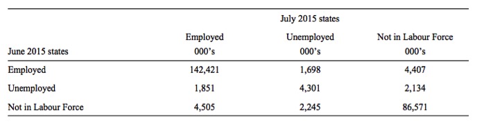
The latest US gross flows data is for transitions between June to July 2015.
To give you some idea of the magnitude of these flows between any given months, the next table summarises the flows for the US labour market for the period between June to July 2015.
By way of example, you read the Table in the following way. 1,851 thousand unemployed workers in June 1015 entered employment in July 2015 (the UE flow) while 1,698 employed workers in June 2015 became unemployed in July 2015 (the EU flow).
The EE, UU, and NN (main diagonal elements) flows just tell us that, for example, 142,421 thousand workers who were employed in June 2015 remained employed in December 2013 (EE flow). The other main diagonal elements (UU, NN) are 4,301 thousand and 86,571 thousand, respectively. These are the unchanged state flows.
It doesn’t mean though that a worker who was employed in June 2015 and remained that way in July 2015, didn’t change jobs. Those type of flows are not captured in this data and can be substantial.
The data also allows us to understand the total change in each state. For example, why did unemployment fall in the US between June and July 2015? Or where did the change in employment come from between these months?
This involves a calculation of the total inflows and outflows from the three labour force states between any two periods of interest.
The following Table shows the concepts total inflows and outflows and total change in state between periods.
The total inflow into employment is measured by the sum, UE + NE and for the period show equalled 6,356 thousand whereas the total outflow from employment, measured by the sum, EU + EN was 6,105 thousand. The net flow was thus positive (that is, employment rose) and equal to 251 thousand workers.
The total inflow into unemployment is measured by the sum, EU + NU and for the period show equalled 3,943 thousand whereas the total outflow from unemployment, measured by the sum, UE + UN was 3,985 thousand. The net flow was thus negative (meaning unemployment fell over the period) and equal to -421 thousand workers.
Finally, the total exits from the labour force is measured by the sum, EN + UN and for the period show equalled 6,541 thousand whereas the total new entrants into the labour force, measured by the sum, NE + NU was 6,750 thousand. The net flow was thus equal to 209 thousand workers extra workers entered the labour force.
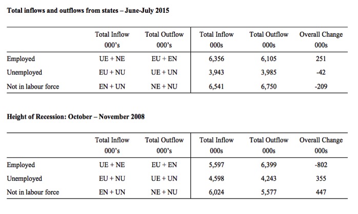
To put the flows for June and July 2015 into context, the lower panel shows what the data looked like at the height of the recession when employment was collapsing – October and November 2008.
You can see that the total change in employment was -802 thousand in the month and 355 thousand of those who lost jobs entered unemployment but 447 thousand left the labour force – early (forced) retirement or discouraged workers.
If the labour force had not contracted then the US unemployment rate would have been much higher than it was (and is). The cyclical shifts in participation mean that the full extent of the labour force underutlisation is disguised and some of it manifests outside of the labour force.
And that doesn’t even consider that of the 5,597 thousand that remained in employment between October and November 2008, many would have been reduced to part-time hours because of lack of sales. That is, this data doesn’t tell us about shifts in underemployment.
We can thus understand the stock measures of the labour market states in each period by considering the net flows between two periods.
To learn more about this please read my blog – Labour market measurement – Part 2.
Transition Probabilities
The various inflows and outflows between the labour force categories are expressed in terms of numbers of persons which can then be converted into so-called transition probabilities – the probabilities that transitions (changes of state) occur.
We can then answer questions like: What is the probability that a person who is unemployed now will enter employment next period?
So if a transition probability for the shift between employment to unemployment is 0.05, we say that a worker who is currently employed has a 5 per cent chance of becoming unemployed in the next month. If this probability fell to 0.01 then we would say that the labour market is improving (only a 1 per cent chance of making this transition).
From the table above – sometimes called a Gross Flows Matrix – we can deduce the gross flows. For example, the element EE tells you how many people who were in employment in the previous month remain in employment in the current month.
Similarly the element EU tells you how many people who were in employment in the previous month are now unemployed in the current month. And so on. This allows you to trace all inflows and outflows from a given state during the month in question.
The transition probabilities are computed by dividing the flow element in the matrix by the initial state. For example, if you want the probability of a worker remaining unemployed between the two months you would divide the flow (UU) by the initial stock of unemployment. If you wanted to compute the probability that a worker would make the transition from employment to unemployment you would divide the flow (EU) by the initial stock of employment. And so on.
So the 3 Labour Force states in the Matrix Table above allow us to compute 9 transition probabilities reflecting the inflows and outflows from each of the combinations.
Analysing movements in these probabilities over time provides a different insight into how the labour market is performing by way of flows of workers.
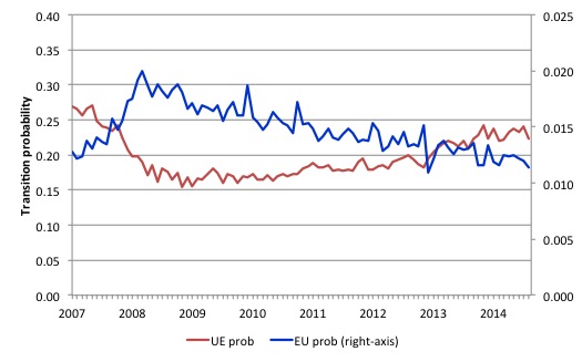
The next graph shows the transitions for EU and UE from December 2007 (when the crisis hit the US labour market) up to July 2015. The probability of an employed worker losing their job (denoted ‘EU prob’ and not to be confused with the Gross Flow from employment to unemployment ‘EU’) is plotted on the right-hand axis and to express the probabilities in percentage terms just multiply by 100.
The probability of an American (in general) losing their job if employed (blue line) rose throughout 2008 (peaking at 2 per cent in February 2009), slowly evened out and has been steadily falling since (1.1 per cent in July 2015). It is now lower than it was when the US entered the crisis.
In December 2007, the chance of an unemployed American worker gaining employment (‘UE prob’) was 27 per cent. This probability fell to a low of 15.4 per cent in October 2009, and scudded along at around 17 per cent through much of 2010-2011. It has been steadily rising since the end of 2013 and is now at 22.3 per cent, still well below the pre-crisis level.
In recent months, this probability has fallen somewhat which is consistent with weaker conditions. Workers in employment are less likely to lose their jobs at present than say at the start of the year but unemployed workers have less chance of getting a job now.
This is not a rapid recovery – rather one would now say the US is in a steady recovery, although the tension has been eased by workers giving up looking for work and exiting the labour market. That is a big difference between this recession and previous recessions where the participation rates were more responsive (positively) to the upturn.
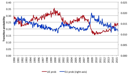
The following graph compares the UE and EU transition probabilities since 1990 to put the recent period into some historical context.
The sharp rises in EU prob and sharp fall in UE prob in 2007-08 are notable and and EU prob is now moving back towards its historical level.
What is also evident is that the employment is becoming more secure (EU prob falling steadily) but the overall real GDP growth rate has not been sufficient to clear out the unemployment pool given the new entrants to the labour force and to attract those who have left the labour force for want of a job. The result is that the UE likelihood improved only slowly and remained well below its historical levels for an extended period.
You can see that in previous periods when the UE probability has dropped the resulting improvement has quickly taken it above the EU probability. But in the tepid recovery that the US is underwent it took a long period to reach the point where a worker has less chance of losing their job and entering unemployment (EU prob) than an unemployed person has of getting a job.
The next graph (or 6 separate graphs) shows the the US transition probabilities from December 2007 (the low-point unemployment rate month of the last cycle) to July 2015 for the 6 transitions (EU, UE, EN, NE, NU, and UN). We exclude the same state probabilities (EE, UU, and NN). Note the vertical scales are different (they are optimised for the particular range of probabilities in each.
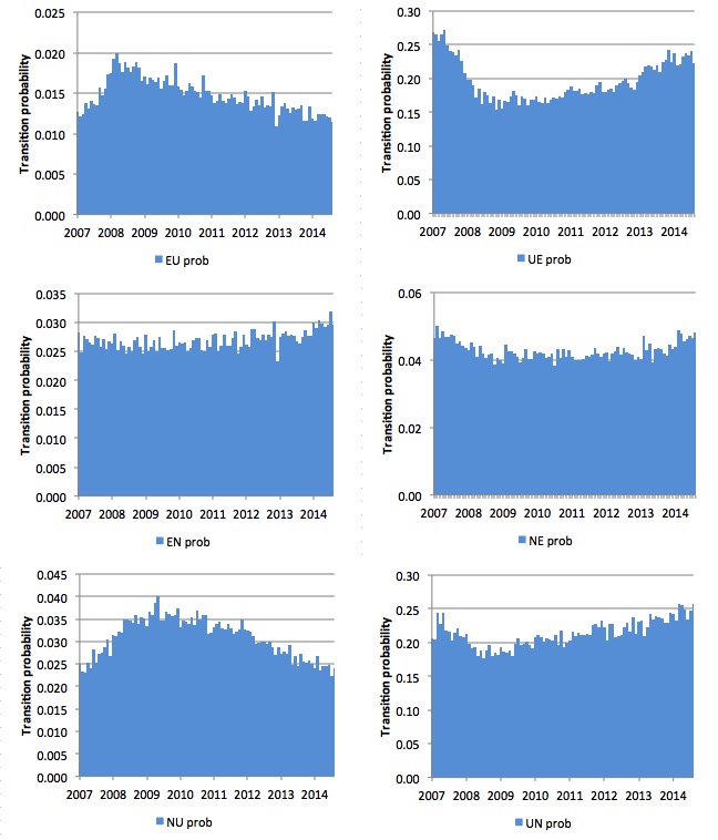
Several points by way of interpretation can be made (noting that care should be taken to recognise the vertical scales are quite different).
First, the EU probability (employment to unemployment) has fallen since the early days of the crisis but is now hovering around 12-13 per cent and is now at 11 per cent and below the pre-crisis value of 13 per cent.
Second, the EN probability has risen marginally indicating that employed workers are now increasingly likely to flow out of the labour force once they lose their jobs – that is, they become hidden unemployed or retire (in some form or another). This is a sign that the labour market is still not very strong.
Third, the likelihood of a new entrant getting a job (NE prob) has risen in recent months after being flat for some months. New entrants are more likely to become employed (NE prob) than enter the labour force unemployed (NU).
Fourth, the probability of an unemployed worker leaving the labour force (UN prob) remains higher than the likelihood of them getting a job (UE prob) although the difference is narrowing.
The former probability has risen over the last 2 years, which is not a good sign (and is consistent with the continued deterioration in the participation rate).
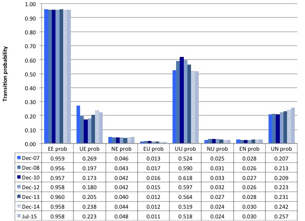
The second graph compares the US transition probabilities for various months during the crisis up until July 2015 (see the accompanying Table for values). I have also jigged the vertical and horizontal scales to allow the changes in the columns to be seen more clearly. That is one of the reasons I also provided the raw data.
December 2007 was the peak of the last cycle and things deteriorated after that. The graph and table give you a year by year summary of how things have changed in the 7.5 years of recession and recovery.
Conclusion
Overall, the Gross Flows data suggests that the US labour market has started to slow a little in mid-2015.
There has been steady improvement but signs of weakness are now showing themselves.
That is enough for today!
(c) Copyright 2015 Bill Mitchell. All Rights Reserved.
Prof. Mitchell,
I think there is a typo in:
“First, the EU probability (employment to unemployment) has fallen since the early days of the crisis but is now hovering around 12-13 per cent and is now at 11 per cent and below the pre-crisis value of 13 per cent.”
and that it should be 1.2 and 1.3 percent etc.
Best Regards,
Will
Dear Willis K (at 2015/08/12 at 1:23)
Thanks for your comment.
The vertical scales can be multiplied by 100 to give a percentage probability.
best wishes
bill