Here are the answers with discussion for this Weekend’s Quiz. The information provided should help you work out why you missed a question or three! If you haven’t already done the Quiz from yesterday then have a go at it before you read the answers. I hope this helps you develop an understanding of Modern…
The Weekend Quiz – August 27-28, 2016 – answers and discussion
Here are the answers with discussion for this Weekend’s Quiz. The information provided should help you work out why you missed a question or three! If you haven’t already done the Quiz from yesterday then have a go at it before you read the answers. I hope this helps you develop an understanding of modern monetary theory (MMT) and its application to macroeconomic thinking. Comments as usual welcome, especially if I have made an error.
Question 1:
Assume that a nation is running an on-going external deficit of 2 per cent of GDP. If the private domestic sector successfully spends less than its income, then we would always find a public sector deficit being recorded.
The answer is True.
This question requires an understanding of the sectoral balances that can be derived from the National Accounts. But it also requires some understanding of the behavioural relationships within and between these sectors which generate the outcomes that are captured in the National Accounts and summarised by the sectoral balances.
Refreshing the balances (again) – we know that from an accounting sense, if the external sector overall is in deficit, then it is impossible for both the private domestic sector and government sector to run surpluses. One of those two has to also be in deficit to satisfy the accounting rules.
The important point is to understand what behaviour and economic adjustments drive these outcomes.
To refresh your memory the balances are derived as follows. The basic income-expenditure model in macroeconomics can be viewed in (at least) two ways: (a) from the perspective of the sources of spending; and (b) from the perspective of the uses of the income produced. Bringing these two perspectives (of the same thing) together generates the sectoral balances.
From the sources perspective we write:
(1) GDP = C + I + G + (X – M)
which says that total national income (GDP) is the sum of total final consumption spending (C), total private investment (I), total government spending (G) and net exports (X – M).
Expression (1) tells us that total income in the economy per period will be exactly equal to total spending from all sources of expenditure.
We also have to acknowledge that financial balances of the sectors are impacted by net government taxes (T) which includes all tax revenue minus total transfer and interest payments (the latter are not counted independently in the expenditure Expression (1)).
Further, as noted above the trade account is only one aspect of the financial flows between the domestic economy and the external sector. we have to include net external income flows (FNI).
Adding in the net external income flows (FNI) to Expression (2) for GDP we get the familiar gross national product or gross national income measure (GNP):
(2) GNP = C + I + G + (X – M) + FNI
To render this approach into the sectoral balances form, we subtract total net taxes (T) from both sides of Expression (3) to get:
(3) GNP – T = C + I + G + (X – M) + FNI – T
Now we can collect the terms by arranging them according to the three sectoral balances:
(4) (GNP – C – T) – I = (G – T) + (X – M + FNI)
The the terms in Expression (4) are relatively easy to understand now.
The term (GNP – C – T) represents total income less the amount consumed less the amount paid to government in taxes (taking into account transfers coming the other way). In other words, it represents private domestic saving.
The left-hand side of Equation (4), (GNP – C – T) – I, thus is the overall saving of the private domestic sector, which is distinct from total household saving denoted by the term (GNP – C – T).
In other words, the left-hand side of Equation (4) is the private domestic financial balance and if it is positive then the sector is spending less than its total income and if it is negative the sector is spending more than it total income.
The term (G – T) is the government financial balance and is in deficit if government spending (G) is greater than government tax revenue minus transfers (T), and in surplus if the balance is negative.
Finally, the other right-hand side term (X – M + FNI) is the external financial balance, commonly known as the current account balance (CAD). It is in surplus if positive and deficit if negative.
In English we could say that:
The private financial balance equals the sum of the government financial balance plus the current account balance.
We can re-write Expression (6) in this way to get the sectoral balances equation:
(5) (S – I) = (G – T) + CAD
which is interpreted as meaning that government sector deficits (G – T > 0) and current account surpluses (CAD > 0) generate national income and net financial assets for the private domestic sector.
Conversely, government surpluses (G – T < 0) and current account deficits (CAD < 0) reduce national income and undermine the capacity of the private domestic sector to add financial assets.
Expression (5) can also be written as:
(6) [(S – I) – CAD] = (G – T)
where the term on the left-hand side [(S – I) – CAD] is the non-government sector financial balance and is of equal and opposite sign to the government financial balance.
This is the familiar MMT statement that a government sector deficit (surplus) is equal dollar-for-dollar to the non-government sector surplus (deficit).
The sectoral balances equation says that total private savings (S) minus private investment (I) has to equal the public deficit (spending, G minus taxes, T) plus net exports (exports (X) minus imports (M)) plus net income transfers.
All these relationships (equations) hold as a matter of accounting and not matters of opinion.
So what economic behaviour might lead to the outcome specified in the question?
If the nation is running an external deficit it means that the contribution to aggregate demand from the external sector is negative – that is net drain of spending – dragging output down. The reference to the specific 2 per cent of GDP figure was to place doubt in your mind. In fact, it doesn’t matter how large or small the external deficit is for this question.
Assume, now that the private domestic sector (households and firms) seeks to increase its saving ratio and is successful in doing so. Consistent with this aspiration, households may cut back on consumption spending and save more out of disposable income. The immediate impact is that aggregate demand will fall and inventories will start to increase beyond the desired level of the firms.
The firms will soon react to the increased inventory holding costs and will start to cut back production. How quickly this happens depends on a number of factors including the pace and magnitude of the initial demand contraction. But if the households persist in trying to save more and consumption continues to lag, then soon enough the economy starts to contract – output, employment and income all fall.
The initial contraction in consumption multiplies through the expenditure system as workers who are laid off also lose income and their spending declines. This leads to further contractions.
The declining income leads to a number of consequences. Net exports improve as imports fall (less income) but the question clearly assumes that the external sector remains in deficit. Total saving actually starts to decline as income falls as does induced consumption.
So the initial discretionary decline in consumption is supplemented by the induced consumption falls driven by the multiplier process.
The decline in income then stifles firms’ investment plans – they become pessimistic of the chances of realising the output derived from augmented capacity and so aggregate demand plunges further. Both these effects push the private domestic balance further towards and eventually into surplus
With the economy in decline, tax revenue falls and welfare payments rise which push the public fiscal balance towards and eventually into deficit via the automatic stabilisers.
If the private sector persists in trying to increase its saving ratio then the contracting income will clearly push the fiscal balance into deficit.
So if there is an external deficit and the private domestic sector saves (a surplus) then there will always be a fiscal deficit. The higher the private saving, the larger the deficit.
The following Graph and related Table shows you the sectoral balances written as (G-T) = (S-I) – (X-M) and how the fiscal deficit rises as the private domestic saving rises.

The following blogs may be of further interest to you:
- Barnaby, better to walk before we run
- Stock-flow consistent macro models
- Norway and sectoral balances
- The OECD is at it again!
Question 2:
The government has to issue debt if the central bank is targetting a non-zero policy rate and is reluctant to pay a return on excess bank reserves.
The answer is True.
I am using the term government here in the Modern Monetary Theory (MMT) sense of the consolidation of the central bank and treasury operations.
Central banks conducts what are called liquidity management operations for two reasons. First, they have to ensure that all private cheques (that are funded) clear and other interbank transactions occur smoothly as part of its role of maintaining financial stability. Second, they must maintain aggregate bank reserves at a level that is consistent with their target policy setting given the relationship between the two.
So operating factors link the level of reserves to the monetary policy setting under certain circumstances. These circumstances require that the return on “excess” reserves held by the banks is below the monetary policy target rate. In addition to setting a lending rate (discount rate), the central bank also sets a support rate which is paid on commercial bank reserves held by the central bank.
Commercial banks maintain accounts with the central bank which permit reserves to be managed and also the clearing system to operate smoothly. In addition to setting a lending rate (discount rate), the central bank also can set a support rate which is paid on commercial bank reserves held by the central bank (which might be zero).
Many countries (such as Australia, Canada and zones such as the European Monetary Union) maintain a default return on surplus reserve accounts (for example, the Reserve Bank of Australia pays a default return equal to 25 basis points less than the overnight rate on surplus Exchange Settlement accounts). Other countries like Japan and the US have typically not offered a return on reserves until the onset of the current crisis.
If the support rate is zero then persistent excess liquidity in the cash system (excess reserves) will instigate dynamic forces which would drive the short-term interest rate to zero unless the government sells bonds (or raises taxes). This support rate becomes the interest-rate floor for the economy.
The short-run or operational target interest rate, which represents the current monetary policy stance, is set by the central bank between the discount and support rate. This effectively creates a corridor or a spread within which the short-term interest rates can fluctuate with liquidity variability. It is this spread that the central bank manages in its daily operations.
In most nations, commercial banks by law have to maintain positive reserve balances at the central bank, accumulated over some specified period. At the end of each day commercial banks have to appraise the status of their reserve accounts. Those that are in deficit can borrow the required funds from the central bank at the discount rate.
Alternatively banks with excess reserves are faced with earning the support rate which is below the current market rate of interest on overnight funds if they do nothing. Clearly it is profitable for banks with excess funds to lend to banks with deficits at market rates. Competition between banks with excess reserves for custom puts downward pressure on the short-term interest rate (overnight funds rate) and depending on the state of overall liquidity may drive the interbank rate down below the operational target interest rate. When the system is in surplus overall this competition would drive the rate down to the support rate.
The main instrument of this liquidity management is through open market operations, that is, buying and selling government debt. When the competitive pressures in the overnight funds market drives the interbank rate below the desired target rate, the central bank drains liquidity by selling government debt. This open market intervention therefore will result in a higher value for the overnight rate. Importantly, we characterise the debt-issuance as a monetary policy operation designed to provide interest-rate maintenance. This is in stark contrast to orthodox theory which asserts that debt-issuance is an aspect of fiscal policy and is required to finance deficit spending.
So the fundamental principles that arise in a fiat monetary system are as follows.
- The central bank sets the short-term interest rate based on its policy aspirations.
- Government spending is independent of borrowing which the latter best thought of as coming after spending.
- Government spending provides the net financial assets (bank reserves) which ultimately represent the funds used by the non-government agents to purchase the debt.
- Budget deficits put downward pressure on interest rates contrary to the myths that appear in macroeconomic textbooks about ‘crowding out’.
- The “penalty for not borrowing” is that the interest rate will fall to the bottom of the “corridor” prevailing in the country which may be zero if the central bank does not offer a return on reserves.
- Government debt-issuance is a “monetary policy” operation rather than being intrinsic to fiscal policy, although in a modern monetary paradigm the distinctions between monetary and fiscal policy as traditionally defined are moot.
Accordingly, debt is issued as an interest-maintenance strategy by the central bank. It has no correspondence with any need to fund government spending. Debt might also be issued if the government wants the private sector to have less purchasing power.
Further, the idea that governments would simply get the central bank to “monetise” treasury debt (which is seen orthodox economists as the alternative “financing” method for government spending) is highly misleading. Debt monetisation is usually referred to as a process whereby the central bank buys government bonds directly from the treasury.
In other words, the federal government borrows money from the central bank rather than the public. Debt monetisation is the process usually implied when a government is said to be printing money. Debt monetisation, all else equal, is said to increase the money supply and can lead to severe inflation.
However, as long as the central bank has a mandate to maintain a target short-term interest rate, the size of its purchases and sales of government debt are not discretionary. Once the central bank sets a short-term interest rate target, its portfolio of government securities changes only because of the transactions that are required to support the target interest rate.
The central bank’s lack of control over the quantity of reserves underscores the impossibility of debt monetisation. The central bank is unable to monetise the federal debt by purchasing government securities at will because to do so would cause the short-term target rate to fall to zero or to the support rate. If the central bank purchased securities directly from the treasury and the treasury then spent the money, its expenditures would be excess reserves in the banking system. The central bank would be forced to sell an equal amount of securities to support the target interest rate.
The central bank would act only as an intermediary. The central bank would be buying securities from the treasury and selling them to the public. No monetisation would occur.
However, the central bank may agree to pay the short-term interest rate to banks who hold excess overnight reserves. This would eliminate the need by the commercial banks to access the interbank market to get rid of any excess reserves and would allow the central bank to maintain its target interest rate without issuing debt.
The following blogs may be of further interest to you:
- Saturday Quiz – May 1, 2010 – answers and discussion
- Understanding central bank operations
- Building bank reserves will not expand credit
- Building bank reserves is not inflationary
- Deficit spending 101 – Part 1
- Deficit spending 101 – Part 2
- Deficit spending 101 – Part 3
Question 3:
Assume that inflation and nominal interest rates are both constant and zero and a country has a public debt to GDP ratio of 100 per cent. The approach taken by those who support fiscal austerity is to run primary fiscal surpluses to stabilise and then reduce the debt ratio. Under the circumstances given, this strategy can still work even if the economy contracts under the burden of the surpluses.
The answer is True.
First, some background theory and conceptual development.
While Modern Monetary Theory (MMT) places no particular importance in the public debt to GDP ratio for a sovereign government, given that insolvency is not an issue, the mainstream debate is dominated by the concept. The unnecessary practice of fiat currency-issuing governments of issuing public debt $-for-$ to match public net spending (deficits) ensures that the debt levels will always rise when there are deficits.
But the rising debt levels do not necessarily have to rise at the same rate as GDP grows. The question is about the debt ratio not the level of debt per se.
Rising deficits often are associated with declining economic activity (especially if there is no evidence of accelerating inflation) which suggests that the debt/GDP ratio may be rising because the denominator is also likely to be falling or rising below trend.
Further, historical experience tells us that when economic growth resumes after a major recession, during which the public debt ratio can rise sharply, the latter always declines again.
It is this endogenous nature of the ratio that suggests it is far more important to focus on the underlying economic problems which the public debt ratio just mirrors.
Mainstream economics starts with the flawed analogy between the household and the sovereign government such that any excess in government spending over taxation receipts has to be “financed” in two ways: (a) by borrowing from the public; and/or (b) by “printing money”.
Neither characterisation is remotely representative of what happens in the real world in terms of the operations that define transactions between the government and non-government sector.
Further, the basic analogy is flawed at its most elemental level. The household must work out the financing before it can spend. The household cannot spend first. The government can spend first and ultimately does not have to worry about financing such expenditure.
However, the mainstream framework for analysing these so-called “financing” choices is called the government budget constraint (GBC). The GBC says that the fiscal deficit in year t is equal to the change in government debt over year t plus the change in high powered money over year t. So in mathematical terms it is written as:
![]()
which you can read in English as saying that Budget deficit = Government spending + Government interest payments – Tax receipts must equal (be “financed” by) a change in Bonds (B) and/or a change in high powered money (H). The triangle sign (delta) is just shorthand for the change in a variable.
However, this is merely an accounting statement. In a stock-flow consistent macroeconomics, this statement will always hold. That is, it has to be true if all the transactions between the government and non-government sector have been correctly added and subtracted.
So in terms of MMT, the previous equation is just an ex post accounting identity that has to be true by definition and has no real economic importance.
But for the mainstream economist, the equation represents an ex ante (before the fact) financial constraint that the government is bound by. The difference between these two conceptions is very significant and the second (mainstream) interpretation cannot be correct if governments issue fiat currency (unless they place voluntary constraints on themselves and act as if it is a financial constraint).
Further, in mainstream economics, money creation is erroneously depicted as the government asking the central bank to buy treasury bonds which the central bank in return then prints money. The government then spends this money.
This is called debt monetisation and you can find out why this is typically not a viable option for a central bank by reading the Deficits 101 suite – Deficit spending 101 – Part 1 – Deficit spending 101 – Part 2 – Deficit spending 101 – Part 3.
Anyway, the mainstream claims that if governments increase the money growth rate (they erroneously call this “printing money”) the extra spending will cause accelerating inflation because there will be “too much money chasing too few goods”! Of-course, we know that proposition to be generally preposterous because economies that are constrained by deficient demand (defined as demand below the full employment level) respond to nominal demand increases by expanding real output rather than prices. There is an extensive literature pointing to this result.
So when governments are expanding deficits to offset a collapse in private spending, there is plenty of spare capacity available to ensure output rather than inflation increases.
But not to be daunted by the “facts”, the mainstream claim that because inflation is inevitable if “printing money” occurs, it is unwise to use this option to “finance” net public spending.
Hence they say as a better (but still poor) solution, governments should use debt issuance to “finance” their deficits. Thy also claim this is a poor option because in the short-term it is alleged to increase interest rates and in the longer-term is results in higher future tax rates because the debt has to be “paid back”.
Neither proposition bears scrutiny – you can read these blogs – Will we really pay higher taxes? and Will we really pay higher interest rates? – for further discussion on these points.
The mainstream textbooks are full of elaborate models of debt pay-back, debt stabilisation etc which all claim (falsely) to “prove” that the legacy of past deficits is higher debt and to stabilise the debt, the government must eliminate the deficit which means it must then run a primary surplus equal to interest payments on the existing debt.
A primary fiscal balance is the difference between government spending (excluding interest rate servicing) and taxation revenue.
The standard mainstream framework, which even the so-called progressives (deficit-doves) use, focuses on the ratio of debt to GDP rather than the level of debt per se. The following equation captures the approach:
![]()
So the change in the debt ratio is the sum of two terms on the right-hand side: (a) the difference between the real interest rate (r) and the GDP growth rate (g) times the initial debt ratio; and (b) the ratio of the primary deficit (G-T) to GDP.
The real interest rate is the difference between the nominal interest rate and the inflation rate.
Many mainstream economists and a fair number of so-called progressive economists say that governments should as some point in the business cycle run primary surpluses (taxation revenue in excess of non-interest government spending) to start reducing the debt ratio back to “safe” territory.
Almost all the media commentators that you read on this topic take it for granted that the only way to reduce the public debt ratio is to run primary surpluses. That is what the whole “credible exit strategy” rhetoric is about and what is driving the austerity push around the world at present.
The standard formula above can easily demonstrate that a nation running a primary deficit can reduce its public debt ratio over time. So it is clear that the public debt ratio can fall even if there is an on-going fiscal deficit if the real GDP growth rate is strong enough. This is win-win way to reduce the public debt ratio.
But the question is analysing the situation where the government is desiring to run primary fiscal surpluses.
Consider the following Table which captures the variations possible in the question. In Year 1, the B/Y(-1) = 1 (that is, the public debt ratio at the start of the period is 100 per cent). The (-1) just signals the value inherited in the current period. We have already assumed that the inflation rate and the nominal interest rate are constant and zero, which means that the real interest rate is also zero and constant. So the r term in the model is 0 throughout our stylised simulation.
This is not to dissimilar to the situation at present in many countries.
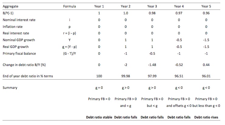
In Year 1, there is zero real GDP growth and the primary fiscal balance (FB) is also zero. Under these circumstances, the debt ratio is stable.
Now in Year 2, the fiscal austerity program begins and assume for the sake of discussion that it doesn’t dent real GDP growth. In reality, a major fiscal contraction is likely to push real GDP growth into the negative (that is, promote a recession). But for the sake of the logic we assume that nominal GDP growth is 1 per cent in Year 2, which means that real GDP growth is also 1 per cent given that all the nominal growth is real (zero inflation).
We assume that the government succeeds in pushing the primary fiscal balance into surplus to 1 per cent of GDP. This is the mainstream nirvana – the public debt ratio falls by 2 per cent as a consequence.
In Year 3, we see that the Primary fiscal surplus remains positive (0.5 per cent of GDP) but is now below the positive real GDP growth rate. In this case the public debt ratio still falls.
In Year 4, real GDP growth contracts (0.5 per cent) and the Primary fiscal surplus remains positive (1 per cent of GDP). In this case the public debt ratio still false which makes the proposition in the question false.
So if you have zero real interest rates, then even in a recession, the public debt ratio can still fall and the government run a fiscal surplus as long as primary fiscal surplus is greater in absolute value to the negative real GDP growth rate. Of-course, this logic is just arithmetic based on the relationship between the flows and stocks involved. In reality, it would be hard for the government to run a primary surplus under these conditions given the automatic stabilisers would be undermining that aim.
In Year 5, the real GDP growth rate is negative 1.5 per cent and the primary fiscal surplus remains positive at 1 per cent of GDP. In this case the public debt ratio rises.
The best way to reduce the public debt ratio is to stop issuing debt. A sovereign government doesn’t have to issue debt if the central bank is happy to keep its target interest rate at zero or pay interest on excess reserves.
The discussion also demonstrates why tightening monetary policy makes it harder for the government to reduce the public debt ratio – which, of-course, is one of the more subtle mainstream ways to force the government to run surpluses.
The following blog may be of further interest to you:
Prof. Mitchell,
I have a question about the “End of year debt ratio in % terms” in the table in question 3. It seems to me that at the end of year two where the debt ratio declined 2% the ending debt ratio would be 98% not 99.98% and so forth for the following years. This does not change the basic answer (True) to the question.
Best Retards,
Willis Kanaley
Bill,
It seems the latest fad in “enlightened left” orthodox economics is to push the idea of Nominal GDP (NGDP) targeting rather than inflation targeting as monetary policy. It seems to me that this might be of marginal help at best in repairing capacity underutilisation in the economy. Is it just another ploy to avoid fiscal stimulus at all costs? What do you think? Is this topic worth a post by you to analyse it?
Dear Ikonoclast (at 2016/08/29 at 9:35 am)
NGDP targetting is just another variant of the obsessive belief that monetary policy is the primary tool for counter stabilisation. I don’t agree with that basic premise and would just neutralise monetary policy and use activist fiscal policy.
That can constitute my blog post on the topic.
best wishes
bill
Bill,
Thanks, that confirms what I suspected about it.