US labour market in an uncertain limbo

Last week, the US Bureau of Labor Statistics released the August 2016 – Employment Situation – which showed that total non-farm employment rose by only 151,000 and the unemployment rate remained steady at 4.9 per cent. Employment growth was well below the expectation (although the banking economists are rarely close) and the question now is being raised as to whether the US has reached a cyclical peak (turning point) and things will get worse from here. While that is difficut to determine on a few months data the fact remains that the US federal government can always offset a slowdown through appropriate fiscal policy interventions if it chooses fit. To dig deeper into the data, I have analysed the Job Openings and Labour Turnover Statistics (JOLTS) which was updated by the BLS yesterday (September 7, 2016). While the number of job openings increased there was little change in the hire and separation rates, which suggests a static situation. In general, it looks as if the US labour market is cooling although perhaps describing the current situation as being an uncertain limbo is more apposite.

Overview

For those who are confused about the difference between the payroll (establishment) data and the household survey data you should read this blog – US labour market is in a deplorable state – where I explain the differences in detail.

See also the – Employment Situation FAQ – provided by the BLS, itself.

The BLS say that:

The establishment survey employment series has a smaller margin of error on the measurement of month-to-month change than the household survey because of its much larger sample size. … However, the household survey has a more expansive scope than the establishment survey because it includes self-employed workers whose businesses are unincorporated, unpaid family workers, agricultural workers, and private household workers …

Focusing on the Household Labour Force Survey data, the seasonally adjusted labour force rose by 176 thousand in August 2016 and the participation rate was stable.

Total employment rose by only 97 thousand in net terms, and as a consequence of the stronger labour force growth, there was a rise in unemployment of 79 thousand.

The unemployment rate rose from 4.88 per cent to 4.92 per cent.

The August participation rate of 62.8 per cent is still 0.2 points below the most recent peak of 63 per cent in March 2016.

Adjusting for the ageing effect (see US labour market – some improvement but still soft for an explanation of this effect), the rise in those who have given up looking for work (discouraged) in the last five months is around 139 thousand workers.

If we added them back into the labour force and considered them to be unemployed (which is not an unreasonable assumption given that the difference between being classified as officially unemployed against not in the labour force is solely due to whether the person had actively searched for work in the previous month) – then the unemployment rate would rise to 5 per cent rather than the current official unemployment rate of 4.9 per cent.

However, if we assessed the impact of the loss of participation since the peak (December 2006 – 66.4 per cent) and adjusted for the ageing effect on participation, we would find that 3,761 thousand workers had exited due to lack of employment opportunities, which would make the current US unemployment rate would be 8.3 per cent if they were added back in to the jobless.

That provides a quite different perspective in the way we assess the US recovery.

Employment growth faltering

In January 2016, employment rose by 0.41 per cent, while the labour force rose by 0.32 per cent. Since then, employment growth has been declining (even negative in April) and the participation rate has fallen back (despite recent stability).

Employment growth in August was a mediocre 0.06 per cent.

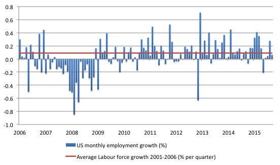
The following graph shows the monthly employment growth since the low-point unemployment rate month (December 2006). The red line is the average labour force growth over the period December 2001 to December 2006 (0.0910 per cent per month). The unemployment rate rises if the employment growth is below the labour force growth rate.

What is apparent is that a strong positive and reinforcing trend in employment growth has not yet been established in the US labour market since the recovery began back in 2009. There are still many months where employment growth, while positive, remains relatively weak when compared to the average labour force growth prior to the crisis.

The weak employment growth since January was interrupted in February and July only. But it is still too early to establish whether that is a new trend or the vagaries of monthly employment data.

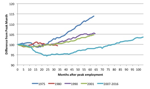
As a matter of history, the following graph shows employment indexes for the US (from US Bureau of Labor Statistics data) for the five NBER recessions since the mid-1970s.

They are indexed at the NBER peak (which doesn’t have to coincide with the employment peak). We trace them out to 64 months or so, except for the first-part of the 1980 downturn which lasted a short period.

It was followed by a second major downturn 12 months later in July 1982 which then endured. In the current period, employment only returned to an index value of 100 in June 2014 (after 78 months). The previous peak was last achieved in December 2007.

The previous recessions have returned to the 100 index value after around 30 to 34 months.

After 104 months, total employment in the US has still only risen by 3.7 per cent (since December 2007), which is a very moderate growth path as is shown in the graph.

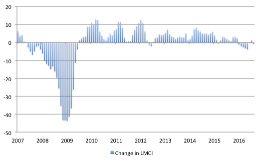
Federal Reserve Bank Labor Market Conditions Index (LMCI)

The Federal Reserve Bank of America has been publishing a new indicator – Labor Market Conditions Index (LMCI) – which is derived from a statistical analysis of 19 individual labour market measures since October 2014.

It is now being watched by those who want to be the first to predict a rise in US official interest rates. Suffice to say that the short-run (monthly) changes in the LMCI are “assumed to summarize overall labor market conditions”.

A rising value (positive change) is a sign of an improving labour market, whereas a declining value (negative change) indicates the opposite.

You can get the full dataset HERE.

I discussed the derivation and interpretation of the LMCI in this blog – US labour market weakening.

The LMCI dropped by 0.7 index points in Auygust 2016, after a positive increase in July. Prior to July, the index had fallen for six consecutive months which signalled a weakening situation.

Whether the July result is an aberration and August has re-established the negative trend is unclear but likely.

The following graph shows the FRB LMCI for the period January 2007 to June 2016.

We note that while unemployment is now lower than last year and the rate of hiring has stabilised after declining earlier in the year. The way these factors combine in the index leads to an overall assessment that the labour market has been in decline.

The fall away over the last eight months has been quite significant notwithstanding the July 2016 upturn.

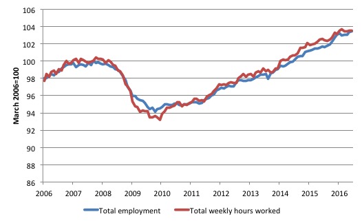
Hours and People in Employment

The next graph shows the index of aggregate weekly hours worked by all employees from March 2006 to August 2016 (red line) and total civilian employment (blue line). The data is from the BLS. Both series are indexed to 100 at December 2007 – the peak employment month before the GFC.

Prior to the crisis, the two series moved more in line with each other as average weekly working hours remained fairly steady.

When the GFC hit, firms adjusted by sacking workers but also reducing hours available, the latter effect being greater because firms hoard skilled labour given the hiring and firing costs are high. The last thing a firm wants to get is a reputation for being capricious when it comes to expensive labour. Such a firm will find it hard attracting skilled labour in the upturn.

As the recovery ensued, both employment in persons and total weekly hours worked rose, the latter more quickly as the hoarded labour was put back onto longer time.

That process does not seem to have fully exhausted itself yet and, in part, explains the relatively slow employment growth rate when measured in persons rather than hours.

Job openings and unemployment

How does this fit in with the hiring and firing data available from the – US JOLTS database – supplied by the BLS.

The JOLTS data allows us to explore the evidence-base to distinguish whether it is ‘supply-side’ movements that are driving the shift in unemployment (that is, actions by workers) or whethor ‘demand-side’ factors are more influential.

In general, the JOLTS database usually always shows that it is the number of jobs on offer and the growth of employment that is the dominant force, which means that independent supply-side shifts (workers agree

For there to be employment there must be spending in the economy and mass unemployment is a sign of deficient spending.

Firms create employment in response to demand for their products. They might be confronted by millions of hungry unemployed workers but they still won’t put them on because there is insufficient demand to justify expanding production.

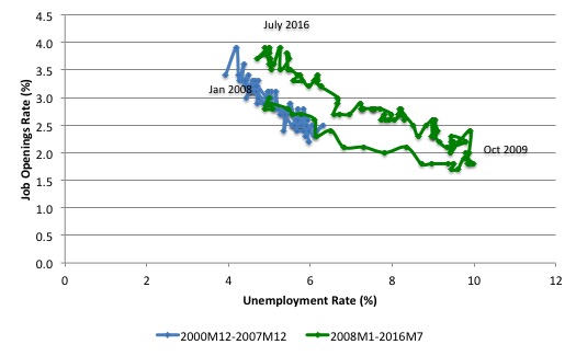
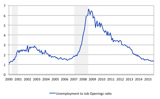
To start the discussion, it is useful to look at the US version of the Unemployment to Vacancies curve (where vacancies are the Total Non-Farm Job Openings as a percent of the Labour Force).

The following graph shows two periods – the first, December 2000 to December 2007, and the second, January 2008 to July 2016. The two periods combined cover the entire span of the JOLTS data. The segments are pre-crisis and post-crisis (where December 2007 was the peak of the last cycle).

Refer to the blog – Latest Australian vacancy data – its all down to deficient demand – for a conceptual discussion about how to interpret this framework in terms of movements along curves and shifts in relationships.

Basically, the UV (or Beveridge) curve shows the unemployment-vacancy (UV) relationship, which plots the unemployment rate on the horizontal axis and the vacancy rate on the vertical axis to investigate these sorts of questions.

The Beveridge curve is named after the British economist William Beveridge who was influential in defining the full employment agenda in the Post World War 2 period in the UK (and, arguably in most advanced nations).

The logic is that movements along the curve are cyclical events and shifts in the curve are alleged to be structural events.

So a movement ‘down along the curve’ to the south-east suggests a decline in the number of jobs available due to an aggregate demand failure, while a movement ‘up along the curve’ indicates improved aggregate demand and lower unemployment.

If unemployment rises in an economy where there are movements along the UV curve it is referred to as “Keynesian” or “cyclical” unemployment – that is, arising from a deficiency in aggregate demand.

The mainstream economics literature claims that ‘shifts in the curve’ – out (in) – indicate non-cyclical (structural) factors are causing the rising (falling) unemployment. Allegedly, the UV curve shifts out because the labour market was becoming less efficient in matching labour supply and labour demand and vice versa for shifts inwards.

The factors that allegedly ’cause’ increasing inefficiency are the usual neo-liberal targets – the provision of income assistance to the unemployed (dole); other welfare payments, trade unions, minimum wages, changing preferences of the workers (poor attitudes to work, laziness, preference for leisure, etc).

The problem is that this view is at odds with the evidence.

As is the case in most advanced countries, the shift in the US curve occurred during a major demand-side recession – that is, it has been driven by cyclical downturns (macroeconomic events) rather than any autonomous supply-side shifts.

Once the economy resumed growth the unemployment rate fell more or less in line with the new job openings rate – tracing the green line up to the north-west of the graph.

It has remained outside the blue curve because employment growth has been subdued in the ‘recovery’ period.

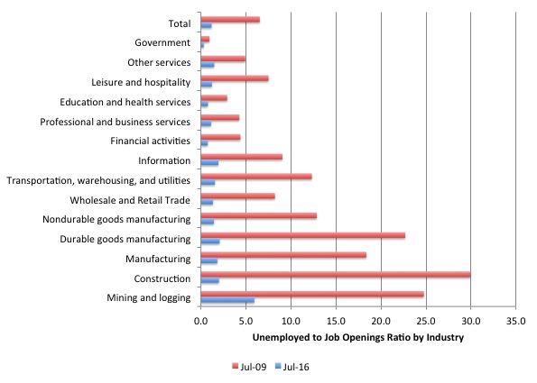
I also examined the sector UV relationships in terms of unemployment-job opening ratios to see where the slack was.

The following graph shows the UV ratios for the aggregated industry sectors (and total All Industries) for two periods: (a) the low-point in the downturn (July 2009) and; (b) the latest month’s observations – July 2016.

There has clearly been dramatic improvement.

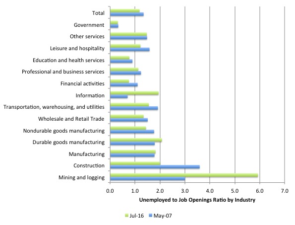
A comparison with the pre-crisis situation (as at May 2007) is presented in the next graph.

The aggregate UV ratio is now slightly lower than it was in May 2007. Industries where there is still significant slack (and worse off than prior to the crisis) include Mining and Logging (5.9 unemployed workers per job opening), Durable goods manufacturing (2.1 unemployed workers per job opening), and Information (1.9 unemployed workers per job opening).

All other sectors are more or less back to where they were in May 2007.

Quit rates

We can also look at the behaviour of the quit rate to judge whether the decline in the unemployment rate is being mostly driven by demand-side or supply-side forces.

Remember that the mainstream text book economics view is that the supply-side dominates as workers exert their free choices between labour and leisure.

The supply-side story starts with the textbook model of the labour market which claims that employment and the real wage are determined in the labour market at the intersection of the labour demand and the labour supply functions.

The equilibrium employment level is constructed as full employment because it suggests that every firm who wants to employ at that real wage can find workers who are willing to work and every worker who is willing to work at that real wage can find an employer willing to employ them.

Frictional unemployment is easily derived from this Classical labour market representation, as is voluntary unemployment.

Holding technology constant, all changes in employment (and hence unemployment) are driven by labour supply shifts. There have been many articles written by key mainstream economists (such as Milton Friedman) that argue that economic cycles are driven by labour supply shifts.

The essence of all these supply shift stories is that the quit rate is constructed as being countercyclical – that is, rise when the economy is in decline and vice-versa – despite all evidence to the contrary.

Quits “are voluntary separations, and measure workers’ willingness or ability to leave the job” (Source)

One such text book story is that the economic cycle swings are characterised by swings in voluntary unemployment. So a downturn in employment (and a rise in unemployment) arises – allegedly – because workers develop a renewed preference for more leisure and less work and the supply of labour at each real wage level thus moves inwards (that is, workers are now less willing to supply the same hours of labour as before at the going real wage).

So workers quit their jobs and head to the beach and relax.

The provision of unemployment benefits – so the story goes – increases the attractiveness of leisure. It is seen as a direct subsidy of non-work.

Upturns in economic activity – so the story goes – is characterised by workers developing a new thirst for work and so the supply curve shifts out again – that is, they are willing to supply more hours of work than before at the same real wage levels. Apparently, they get sick of leisure and gain a new appetite for income so as to buy goods and services unattainable while they spent their time in non-work.

And at the empirical level this theory predicts that quits will fall as employment falls.

The simplest fact then, which would give support to this notion of supply-side shifts, is whether the quit rate is, indeed, counter-cyclical – as the theory predicts. That is, does the quit rate rise when the unemployment rate rises or not. Simple enough.

Lester Thurow in his 1983 book – Dangerous Currents – challenged the mainstream view by asking:

… why do quits rise in booms and fall in recessions? If recessions are due to informational mistakes, quits should rise in recessions and fall in booms, just the reverse of what happens in the real world.

The reference to “informational mistakes” is another version of the mainstream supply-side story. The narrative goes that the central bank/treasury can temporarily buy a reduction in unemployment (below what the neo-liberals refer to as the natural rate – another myth) – by inflating the economy with spending.

As economic activity picks up both money wages and prices rise (typical story about too much money chasing too few goods). The trick is that they claim that the rate of increase in money wages is less than the rise in prices and so the real wage falls.

Firms react to the declining real wage by offering more employment – because they know that marginal labour productivity is lower (another myth).

But why do workers agree to supply more labour when the real wage is falling? After all the textbook labour market model tells us that the labour supply curve is upward sloping in terms of the real wage because workers will only supply more labour if the relative price of leisure (which is the real wage) rises.

The trick is that the entire supply of labour shifts because workers think that the real wage has risen – they get beguiled by the rise in money wages into forming the view that they are better off per hour than before and so the quit rate falls and employment increases.

Hence, for a time (a short time), the economy can operate at unemployment levels lower than the natural rate.

How long can this go on for? Well, how long does it take for workers to go down to the shops and realise that everything is more expensive now and, in fact, they are worse off than before (because the real wage has fallen)?

Accordingly, as the story goes, once they learn the truth, the labour supply curve shifts back in and workers withdraw their labour en masse (the quit rate rises again) and employment and economic activity falls back to the ‘natural’ level.

The lesson that is hammered hometo students that this all demonstrates how futile policy interventions that aim to lower the unemployment rate are. The only way the ‘natural’ rate can be lowered (if at all) is for policies to be designed with reduce structural impediments in the labour market. What are they? For example, cut the subsidy to leisure (the unemployment benefit). etc.

It is an extraordinary story in total denial of the facts – but it survives because of the dominance of Groupthink in the academy.

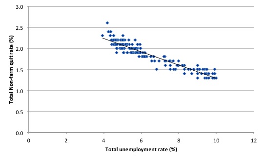
The US Bureau of Labour Market JOLTS database includes estimates of the quit rate. The following graph shows in a compelling way that the quit rate (non-farm quits as a percent of total non-farm employment) behaves in a cyclical fashion as we would expect – that is, it rises when times are good and falls when times are bad.

The graph relates the quit rate (vertical axis) to the unemployment rate (horizontal axis). The straight black line is a simple linear regression trend drawn through the graph.

There are no shifts evident in this relationship just movements along a fairly defined inverse relationship.

That is, when the unemployment rate rises, the quit rate falls. Exactly the opposite to that predicted by the supply-side story which means that their claim that causality runs from unemployment benefits to higher quits to higher unemployment is unsustainable.

Many studies, which are not caught up in the orthodox Groupthink, have demonstrated the phenomenon depicted in this graph – for several countries where decent data is available.

Workers become very cautious when unemployment starts to rise and postpone any desired or planned job changes and opt for the security of their present job.

When there are more jobs being created and the hiring rate rises, workers then take more risks and the quit rate tends to rise.

This also helps us understand why the unemployment-job vacancies graph (above) shifted upwards during the recession and then stabilised as the economy grew again. Remember, that firms were adjusting hours more quickly than persons.

The BLS Monthly Labor Review article (June 15, 2015) – Job openings reach a new high, hires and quits also increase – notes that:

Quits are procyclical, rising during an expansion and falling during a contraction … As of 2014, quits had not reached prerecession values in most industries. While some industries recovered fully to surpass 2007 values, overall, the annual quits level was 88 percent of its 2007 level.

By July 2016, the quit rate of 2.1 is still around 91 per cent of the pre-crisis peak of 2.3, but is higher than it was this time last year.

The US labour market is steadying rather than recovering fast.

The following graph shows the total number of unemployed per job opening (non-farm and seasonally adjusted) and thus gives a measure of how strong the demand-side of the labour market (job openings) is relative to the number of people seeking work (the unemployed).

It is an alternative way of presenting the relationships between unemployment and vacancies.

The shaded area indicates the NBER recession months.

The US Bureau of Labor Statistics (in the article cited) described the data at that point in this way:

The job openings and unemployment levels generally move in opposite directions. During a robust economy, job openings are high and unemployment is low. During an economic contraction, the dynamics reverse – unemployment rises, while job openings fall. Accordingly, the ratio of the unemployed to job openings provides a metric that helps describe the state of the economy … Since July 2009, 1 month after the end of the recession, this ratio has trended downward. In January 2014, the ratio stood at 2.6. By December 2014, it had fallen to 1.8, the same ratio present in December 2007, the start of the recession.

In July 2016, the ratio stood at 1.3 and the rate of decline has been steady albeit slow. It is now below the pre-crisis level.

Labour markets typically behave over the business cycle in an asymmetric manner as can be seen from the graph. The deterioration was sharp and rapid. The recovery is much slower and is all the more slow as the employment growth not only has to absorb new labour force entrants (arising from population growth) but also has to face the huge pool of unemployed that is caused by the recession.

One of the facts I repeat often is that the unemployed cannot search for jobs that are not there! This is exactly what happens when aggregate demand falls and job openings dry up.

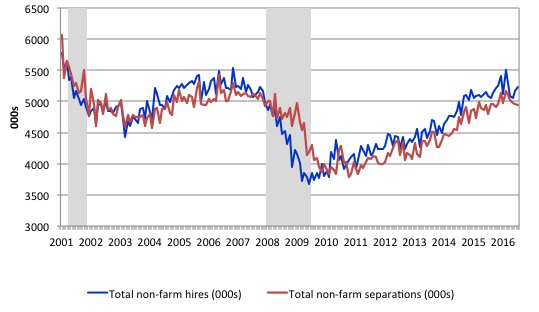
Another way of seeing how the job flows tell us about the direction of change is to compare movements in hires and separations. The following graph shows this relationship for the US economy as published by the BLS for the period from December 2000 to July 2016.

While labour markets are clearly dynamic in the sense that even in a downturn new jobs are being continually created and destroyed the rates of each dynamic change in a cyclical way. So while there were new jobs being created at the height of the downturn there was a severe shortfall of new jobs emerging as is shown in the graph.

Separations also fall for reasons noted above. The difference between hires and separations is the net change in employment in each month. If hires outstrip separations, employment grows and vice versa.

The most recent data shows that hiring and separations have stalled somewhat and even fallen from the levels attained earlier in the year.

The net change in employment per month which began to slowdown in 2015 when compared to 2014 when employment growth was more robust, has continued to stall in 2016.

Whether this is the beginning of a new downturn is unclear at this stage. But it is starting to look like a turning point in the time series.

Further, the layoff and discharges rate also published in the BLS JOLTS database which reflects the demand-side of the labour market is also firmly counter-cyclical as we would expect. Firms layoff workers when there is deficient aggregate demand and hire again when sales pick-up.

Again this is contrary to the mainstream text book logic.

The last graph shows job openings and unemployment from December 2000 to July 2016 (in 000s). Total unemployment (green line) is on the right-axis while total non-farm job openings (blue line) are on the left-axis.

As the economy faltered, job openings collapsed and unemployment rose but not as much as would be predicted by the employment losses.

Why? Answer: Some workers gave up looking and left the labour force. As the job openings increased again in recent months, unemployment has been steady because the discouraged workers are now re-entering the labour force again.

This is accounted for by the significant fall in the US participation rate that is independent of demographic factors such as ageing.

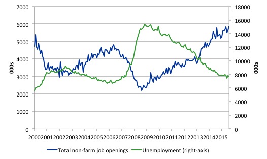
All the evidence supports the conclusion that deficient demand not only increases unemployment in the downturn but also pushes people out of the labour force as they give up actively looking for work that is not there. These hidden unemployed workers re-enter the labour force as the probability of getting a job (in their mind) increases.

Conclusion

Anyway, a bit of a data excursion to complete the day.

The JOLTS data is very useful because it addresses some of the most simple claims made by the mainstream approach to unemployment. And the evidence is clear. There is no validity in the supply-side case that mass unemployment is somehow something to do with the unemployed being lured into leisure by excessive unemployment benefits or some other reason.

The evidence is consistent and strong – the mass unemployment in the US is the result of a systemic failure in that economy to produce enough jobs, which emerged as aggregate spending collapsed in early 2008.

Since then, as the economy has slowly starting growing again, the demand-side of the labour market has improved steadily and the unemployment rate has fallen.

The pace of improvement appears to be slowing.

There is also a debate about how far the US unemployment rate can fall – I will return to that question another day.

That is enough for today!

(c) Copyright 2016 William Mitchell. All Rights Reserved.