Here are the answers with discussion for this Weekend’s Quiz. The information provided should help you work out why you missed a question or three! If you haven’t already done the Quiz from yesterday then have a go at it before you read the answers. I hope this helps you develop an understanding of Modern…
The Weekend Quiz – April 14-15, 2018 – answers and discussion
Here are the answers with discussion for this Weekend’s Quiz. The information provided should help you work out why you missed a question or three! If you haven’t already done the Quiz from yesterday then have a go at it before you read the answers. I hope this helps you develop an understanding of modern monetary theory (MMT) and its application to macroeconomic thinking. Comments as usual welcome, especially if I have made an error.
Question 1:
Assume that the external deficit of a nation is on average over the economic cycle equal to 2 per cent of GDP and that the government balances its fiscal position when averaged over the same cycle. We can conclude that on average the private domestic sector overall:
(a) Is spending more than it is earning.
(b) Is spending less that it is earning.
(c) Cannot say for sure as we don’t know the pattern of fiscal balances over the cycle.
The answer is Option (a) Is spending more than it is earning..
Note that this question doesn’t investigate how the economy might get into this situation. But whatever behavioural forces were at play, the sectoral balances all have to sum to zero. Once you understand that, then deduction leads to the correct answer.
To refresh your memory the balances are derived as follows. The basic income-expenditure model in macroeconomics can be viewed in (at least) two ways: (a) from the perspective of the sources of spending; and (b) from the perspective of the uses of the income produced. Bringing these two perspectives (of the same thing) together generates the sectoral balances.
From the sources perspective we write:
(1) GDP = C + I + G + (X – M)
which says that total national income (GDP) is the sum of total final consumption spending (C), total private investment (I), total government spending (G) and net exports (X – M).
Expression (1) tells us that total income in the economy per period will be exactly equal to total spending from all sources of expenditure.
We also have to acknowledge that financial balances of the sectors are impacted by net government taxes (T) which includes all tax revenue minus total transfer and interest payments (the latter are not counted independently in the expenditure Expression (1)).
Further, as noted above the trade account is only one aspect of the financial flows between the domestic economy and the external sector. we have to include net external income flows (FNI).
Adding in the net external income flows (FNI) to Expression (2) for GDP we get the familiar gross national product or gross national income measure (GNP):
(2) GNP = C + I + G + (X – M) + FNI
To render this approach into the sectoral balances form, we subtract total net taxes (T) from both sides of Expression (3) to get:
(3) GNP – T = C + I + G + (X – M) + FNI – T
Now we can collect the terms by arranging them according to the three sectoral balances:
(4) (GNP – C – T) – I = (G – T) + (X – M + FNI)
The the terms in Expression (4) are relatively easy to understand now.
The term (GNP – C – T) represents total income less the amount consumed less the amount paid to government in taxes (taking into account transfers coming the other way). In other words, it represents private domestic saving.
The left-hand side of Equation (4), (GNP – C – T) – I, thus is the overall saving of the private domestic sector, which is distinct from total household saving denoted by the term (GNP – C – T).
In other words, the left-hand side of Equation (4) is the private domestic financial balance and if it is positive then the sector is spending less than its total income and if it is negative the sector is spending more than it total income.
The term (G – T) is the government financial balance and is in deficit if government spending (G) is greater than government tax revenue minus transfers (T), and in surplus if the balance is negative.
Finally, the other right-hand side term (X – M + FNI) is the external financial balance, commonly known as the current account balance (CAD). It is in surplus if positive and deficit if negative.
In English we could say that:
The private financial balance equals the sum of the government financial balance plus the current account balance.
We can re-write Expression (6) in this way to get the sectoral balances equation:
(5) (S – I) = (G – T) + CAD
which is interpreted as meaning that government sector deficits (G – T > 0) and current account surpluses (CAD > 0) generate national income and net financial assets for the private domestic sector.
Conversely, government surpluses (G – T < 0) and current account deficits (CAD < 0) reduce national income and undermine the capacity of the private domestic sector to add financial assets.
Expression (5) can also be written as:
(6) [(S – I) – CAD] = (G – T)
where the term on the left-hand side [(S – I) – CAD] is the non-government sector financial balance and is of equal and opposite sign to the government financial balance.
This is the familiar MMT statement that a government sector deficit (surplus) is equal dollar-for-dollar to the non-government sector surplus (deficit).
The sectoral balances equation says that total private savings (S) minus private investment (I) has to equal the public deficit (spending, G minus taxes, T) plus net exports (exports (X) minus imports (M)) plus net income transfers.
All these relationships (equations) hold as a matter of accounting and not matters of opinion.
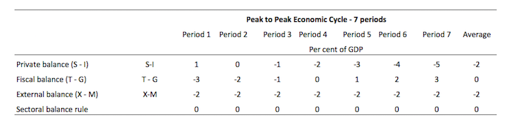
To help us answer the specific question posed, the following Table shows a stylised economic cycle of 7 periods (peak to peak).
The economy is running a fiscal deficit in the first three periods (but declining), a balance in Period 4 and then increasing surpluses. Over the entire cycle the balanced fiscal rule would be achieved as the fiscal balances is on average equal to zero. So the deficits are covered by fully offsetting surpluses over the cycle.
The simplification is the constant external deficit (that is, no cyclical sensitivity) of 2 per cent of GDP over the entire cycle.
You can then see what the private domestic balance is doing clearly. When the fiscal deficit is lower than the external deficit, the private balance is in deficit. The larger the fiscal surplus the larger the private deficit for a given external deficit.
When the fiscal deficit is large enough (3 per cent of GDP) to offset the demand-draining external deficit (2 per cent of GDP), the private domestic sector can save overall. The fiscal deficits allow income growth to be sufficient to generate savings greater than investment in the private domestic sector.
Under the conditions specified in the question, on average over the cycle, the private domestic deficit exactly equals the external deficit. This could be achieved via increasing indebtedness or running down previous savings or asset accumulation.
The following blogs may be of further interest to you:
- Barnaby, better to walk before we run
- Stock-flow consistent macro models
- Norway and sectoral balances
- The OECD is at it again!
Question 2:
Trade unions that manage to push aggregate wages growth ahead of the inflation rate will ensure that workers gain a greater share of national income.
The answer is False.
Workers may enjoy a rising wage share as real wages rise but not necessarily.
The wage share in nominal GDP is expressed as the total wage bill as a percentage of nominal GDP. Economists differentiate between nominal GDP ($GDP), which is total output produced at market prices and real GDP (GDP), which is the actual physical equivalent of the nominal GDP. We will come back to that distinction soon.
To compute the wage share we need to consider total labour costs in production and the flow of production ($GDP) each period.
Employment (L) is a stock and is measured in persons (averaged over some period like a month or a quarter or a year.
The wage bill is a flow and is the product of total employment (L) and the average wage (w) prevailing at any point in time. Stocks (L) become flows if it is multiplied by a flow variable (W). So the wage bill is the total labour costs in production per period.
So the wage bill = W.L
The wage share is just the total labour costs expressed as a proportion of $GDP – (W.L)/$GDP in nominal terms, usually expressed as a percentage. We can actually break this down further.
Labour productivity (LP) is the units of real GDP per person employed per period. Using the symbols already defined this can be written as:
LP = GDP/L
so it tells us what real output (GDP) each labour unit that is added to production produces on average.
We can also define another term that is regularly used in the media – the real wage – which is the purchasing power equivalent on the nominal wage that workers get paid each period. To compute the real wage we need to consider two variables: (a) the nominal wage (W) and the aggregate price level (P).
We might consider the aggregate price level to be measured by the consumer price index (CPI) although there are huge debates about that. But in a sense, this macroeconomic price level doesn’t exist but represents some abstract measure of the general movement in all prices in the economy.
Macroeconomics is hard to learn because it involves these abstract variables that are never observed – like the price level, like “the interest rate” etc. They are just stylisations of the general tendency of all the different prices and interest rates.
Now the nominal wage (W) – that is paid by employers to workers is determined in the labour market – by the contract of employment between the worker and the employer. The price level (P) is determined in the goods market – by the interaction of total supply of output and aggregate demand for that output although there are complex models of firm price setting that use cost-plus mark-up formulas with demand just determining volume sold. We shouldn’t get into those debates here.
The inflation rate is just the continuous growth in the price level (P). A once-off adjustment in the price level is not considered by economists to constitute inflation.
So the real wage (w) tells us what volume of real goods and services the nominal wage (W) will be able to command and is obviously influenced by the level of W and the price level. For a given W, the lower is P the greater the purchasing power of the nominal wage and so the higher is the real wage (w).
We write the real wage (w) as W/P. So if W = 10 and P = 1, then the real wage (w) = 10 meaning that the current wage will buy 10 units of real output. If P rose to 2 then w = 5, meaning the real wage was now cut by one-half.
So the proposition in the question – that nominal wages grow faster than inflation – tells us that the real wage is rising.
Nominal GDP ($GDP) can be written as P.GDP, where the P values the real physical output.
Now if you put of these concepts together you get an interesting framework. To help you follow the logic here are the terms developed and be careful not to confuse $GDP (nominal) with GDP (real):
- Wage share = (W.L)/$GDP
- Nominal GDP: $GDP = P.GDP
- Labour productivity: LP = GDP/L
- Real wage: w = W/P
By substituting the expression for Nominal GDP into the wage share measure we get:
Wage share = (W.L)/P.GDP
In this area of economics, we often look for alternative way to write this expression – it maintains the equivalence (that is, obeys all the rules of algebra) but presents the expression (in this case the wage share) in a different “view”.
So we can write as an equivalent:
Wage share – (W/P).(L/GDP)
Now if you note that (L/GDP) is the inverse (reciprocal) of the labour productivity term (GDP/L). We can use another rule of algebra (reversing the invert and multiply rule) to rewrite this expression again in a more interpretable fashion.
So an equivalent but more convenient measure of the wage share is:
Wage share = (W/P)/(GDP/L) – that is, the real wage (W/P) divided by labour productivity (GDP/L).
I won’t show this but I could also express this in growth terms such that if the growth in the real wage equals labour productivity growth the wage share is constant. The algebra is simple but we have done enough of that already.
That journey might have seemed difficult to non-economists (or those not well-versed in algebra) but it produces a very easy to understand formula for the wage share.
Two other points to note. The wage share is also equivalent to the real unit labour cost (RULC) measures that Treasuries and central banks use to describe trends in costs within the economy. Please read my blog – Saturday Quiz – May 15, 2010 – answers and discussion – for more discussion on this point.
Now it becomes obvious that if the nominal wage (W) grows faster than the price level (P) then the real wage is growing. But that doesn’t automatically lead to a growing wage share. So the blanket proposition stated in the question is false.
If the real wage is growing at the same rate as labour productivity, then both terms in the wage share ratio are equal and so the wage share is constant.
If the real wage is growing but labour productivity is growing faster, then the wage share will fall.
Only if the real wage is growing faster than labour productivity, will the wage share rise.
Question 3:
Sovereign government spending becomes more expensive when government bond yields for new issues rise.
The answer is False.
For a sovereign government that issues its own currency there is no binding revenue constraint on government spending. The interest servicing payments come from the same source as all government spending – its infinite (minus one cent!) capacity to issue fiat currency. There is no “cost” – in real terms to the government doing this.
The concept of more or less expensive is therefore inapplicable to government spending.
The cost of government spending is the real resources that are deployed in the production of the goods and services being purchased rather than the accounting entry in the Treasury books.
Rising bond yields do not measure these opportunity costs.
In macroeconomics, we summarise the plethora of public debt instruments with the concept of a bond. The standard bond has a face value – say $A1000 and a coupon rate – say 5 per cent and a maturity – say 10 years. This means that the bond holder will will get $50 dollar per annum (interest) for 10 years and when the maturity is reached they would get $1000 back.
Bonds are issued by government into the primary market, which is simply the institutional machinery via which the government sells debt to “raise funds”. In a modern monetary system with flexible exchange rates it is clear the government does not have to finance its spending so the the institutional machinery is voluntary and reflects the prevailing neo-liberal ideology – which emphasises a fear of fiscal excesses rather than any intrinsic need.
Once bonds are issued they are traded in the secondary market between interested parties. Clearly secondary market trading has no impact at all on the volume of financial assets in the system – it just shuffles the wealth between wealth-holders. In the context of public debt issuance – the transactions in the primary market are vertical (net financial assets are created or destroyed) and the secondary market transactions are all horizontal (no new financial assets are created). Please read my blog – Deficit spending 101 – Part 3 – for more discussion on this point.
Further, most primary market issuance is now done via auction. Accordingly, the government would determine the maturity of the bond (how long the bond would exist for), the coupon rate (the interest return on the bond) and the volume (how many bonds) being specified.
The issue would then be put out for tender and the market then would determine the final price of the bonds issued. Imagine a $1000 bond had a coupon of 5 per cent, meaning that you would get $50 dollar per annum until the bond matured at which time you would get $1000 back.
Imagine that the market wanted a yield of 6 per cent to accommodate risk expectations (inflation or something else). So for them the bond is unattractive and they would avoid it under the tap system. But under the tender or auction system they would put in a purchase bid lower than the $1000 to ensure they get the 6 per cent return they sought.
The mathematical formulae to compute the desired (lower) price is quite tricky and you can look it up in a finance book.
The general rule for fixed-income bonds is that when the prices rise, the yield falls and vice versa. Thus, the price of a bond can change in the market place according to interest rate fluctuations.
When interest rates rise, the price of previously issued bonds fall because they are less attractive in comparison to the newly issued bonds, which are offering a higher coupon rates (reflecting current interest rates).
When interest rates fall, the price of older bonds increase, becoming more attractive as newly issued bonds offer a lower coupon rate than the older higher coupon rated bonds.
Further, rising yields may indicate a rising sense of risk (mostly from future inflation although sovereign credit ratings will influence this). But they may also indicated a recovering economy where people are more confidence investing in commercial paper (for higher returns) and so they demand less of the “risk free” government paper.
So you see how an event (yield rises) that signifies growing confidence in the real economy is reinterpreted (and trumpeted) by the conservatives to signal something bad (crowding out). In this case, the reason long-term yields would be rising is because investors were diversifying their portfolios and moving back into private financial assets. The yield reflects the last auction bid in the bond issue. So if diversification is occurring reflecting confidence and the demand for public debt weakens and yields rise this has nothing at all to do with a declining pool of funds being soaked up by the binging government!
But all of that has nothing to do with the real resource costs embodied in goods and services that governments purchase.
The following blogs may be of further interest to you:
- Saturday Quiz – April 17, 2010 – answers and discussion
- Time to outlaw the credit rating agencies
- Studying macroeconomics – an exercise in deception
- Time for a reality check on debt – Part 1
- Will we really pay higher interest rates?
That is enough for today!
(c) Copyright 2018 William Mitchell. All Rights Reserved.
Right – I think I finally conquered the algebra of the wage share. Paper, pen, strong coffee, early morning peace and some hypothetical numbers to manipulate (will most likely forget it by next week). One thing a bit confusing – at the start of the explanation the average wage is defined as lower case w – and then it becomes the real wage later on. Should the average wage be upper case “W” at the start too?