Here are the answers with discussion for this Weekend’s Quiz. The information provided should help you work out why you missed a question or three! If you haven’t already done the Quiz from yesterday then have a go at it before you read the answers. I hope this helps you develop an understanding of Modern…
The Weekend Quiz – June 2-3, 2018 – answers and discussion
Here are the answers with discussion for this Weekend’s Quiz. The information provided should help you work out why you missed a question or three! If you haven’t already done the Quiz from yesterday then have a go at it before you read the answers. I hope this helps you develop an understanding of modern monetary theory (MMT) and its application to macroeconomic thinking. Comments as usual welcome, especially if I have made an error.
Question 1:
Start from a situation where the external surplus is the equivalent of 2 per cent of GDP and the fiscal surplus is 2 per cent. If the fiscal balance stays constant and the external surplus rises to the equivalent of 4 per cent of GDP then:
(a) National income rises and the private surplus moves from 4 per cent of GDP to 6 per cent of GDP.
(b) National income remains unchanged and the private surplus moves from 4 per cent of GDP to 6 per cent of GDP.
(c) National income falls and the private surplus moves from 4 per cent of GDP to 6 per cent of GDP.
(d) National income rises and the private surplus moves from 0 per cent of GDP to 2 per cent of GDP.
(e) National income remains unchanged and the private surplus moves from 0 per cent of GDP to 2 per cent of GDP
(f) National income falls and the private surplus moves from 0 per cent of GDP to 2 per cent of GDP.
The answer is Option (d) National income rises and the private surplus moves from 0 per cent of GDP to 2 per cent of GDP.
To refresh your memory the balances are derived as follows. The basic income-expenditure model in macroeconomics can be viewed in (at least) two ways: (a) from the perspective of the sources of spending; and (b) from the perspective of the uses of the income produced. Bringing these two perspectives (of the same thing) together generates the sectoral balances.
From the sources perspective we write:
(1) GDP = C + I + G + (X – M)
which says that total national income (GDP) is the sum of total final consumption spending (C), total private investment (I), total government spending (G) and net exports (X – M).
Expression (1) tells us that total income in the economy per period will be exactly equal to total spending from all sources of expenditure.
We also have to acknowledge that financial balances of the sectors are impacted by net government taxes (T) which includes all tax revenue minus total transfer and interest payments (the latter are not counted independently in the expenditure Expression (1)).
Further, as noted above the trade account is only one aspect of the financial flows between the domestic economy and the external sector. we have to include net external income flows (FNI).
Adding in the net external income flows (FNI) to Expression (2) for GDP we get the familiar gross national product or gross national income measure (GNP):
(2) GNP = C + I + G + (X – M) + FNI
To render this approach into the sectoral balances form, we subtract total net taxes (T) from both sides of Expression (3) to get:
(3) GNP – T = C + I + G + (X – M) + FNI – T
Now we can collect the terms by arranging them according to the three sectoral balances:
(4) (GNP – C – T) – I = (G – T) + (X – M + FNI)
The the terms in Expression (4) are relatively easy to understand now.
The term (GNP – C – T) represents total income less the amount consumed less the amount paid to government in taxes (taking into account transfers coming the other way). In other words, it represents private domestic saving.
The left-hand side of Equation (4), (GNP – C – T) – I, thus is the overall saving of the private domestic sector, which is distinct from total household saving denoted by the term (GNP – C – T).
In other words, the left-hand side of Equation (4) is the private domestic financial balance and if it is positive then the sector is spending less than its total income and if it is negative the sector is spending more than it total income.
The term (G – T) is the government financial balance and is in deficit if government spending (G) is greater than government tax revenue minus transfers (T), and in surplus if the balance is negative.
Finally, the other right-hand side term (X – M + FNI) is the external financial balance, commonly known as the current account balance (CAD). It is in surplus if positive and deficit if negative.
In English we could say that:
The private financial balance equals the sum of the government financial balance plus the current account balance.
We can re-write Expression (6) in this way to get the sectoral balances equation:
(5) (S – I) = (G – T) + CAD
which is interpreted as meaning that government sector deficits (G – T > 0) and current account surpluses (CAD > 0) generate national income and net financial assets for the private domestic sector.
Conversely, government surpluses (G – T < 0) and current account deficits (CAD < 0) reduce national income and undermine the capacity of the private domestic sector to add financial assets.
Expression (5) can also be written as:
(6) [(S – I) – CAD] = (G – T)
where the term on the left-hand side [(S – I) – CAD] is the non-government sector financial balance and is of equal and opposite sign to the government financial balance.
This is the familiar MMT statement that a government sector deficit (surplus) is equal dollar-for-dollar to the non-government sector surplus (deficit).
The sectoral balances equation says that total private savings (S) minus private investment (I) has to equal the public deficit (spending, G minus taxes, T) plus net exports (exports (X) minus imports (M)) plus net income transfers.
All these relationships (equations) hold as a matter of accounting and not matters of opinion.
Thus, when an external deficit (X – M < 0) and public surplus (G – T < 0) coincide, there must be a private domestic deficit. While private spending can persist for a time under these conditions using the net savings of the external sector, the private sector becomes increasingly indebted in the process.
Second, you then have to appreciate the relative sizes of these balances to answer the question correctly.
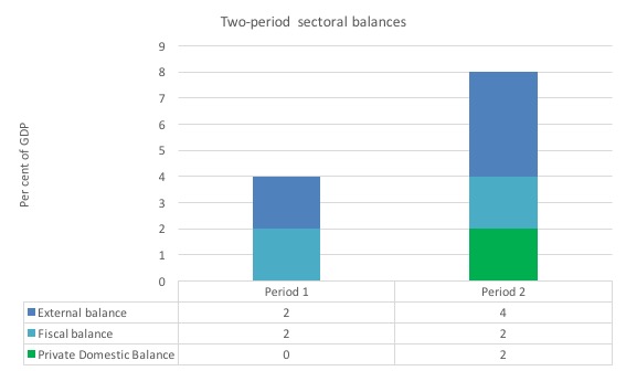
Consider the following graph and accompanying table which depicts two periods outlined in the question.
In Period 1, with an external surplus of 2 per cent of GDP and a fiscal surplus of 2 per cent of GDP the private domestic balance is zero. The demand injection from the external sector is exactly offset by the demand drain (the fiscal drag) coming from the fiscal balance and so the private sector can neither net save or spend more than they earn.
In Period 2, with the external sector adding more to demand now – surplus equal to 4 per cent of GDP and the fiscal balance unchanged (this is stylised – in the real world the fiscal balance will certainly change), there is a stimulus to spending and national income would rise.
The rising national income also provides the capacity for the private sector to save overall and so they can now save 2 per cent of GDP.
The fiscal drag is overwhelmed by the rising net exports.
This is a highly stylised example and you could tell a myriad of stories that would be different in description but none that could alter the basic point.
If the drain on spending (from the public sector) is more than offset by an external demand injection, then GDP rises and the private sector overall saving increases.
If the drain on spending from fsical policy outweighs the external injections into the spending stream then GDP falls (or growth is reduced) and the overall private balance would fall into deficit.
You may wish to read the following blogs for more information:
- Back to basics – aggregate demand drives output
- Stock-flow consistent macro models
- Norway and sectoral balances
- The OECD is at it again!
- Barnaby, better to walk before we run
- Saturday Quiz – June 19, 2010 – answers and discussion
Question 2:
A rising fiscal deficit tells us that the government is pursuing an increasingly expansionary fiscal stance.
The answer is False.
The actual fiscal deficit outcome that is reported in the press and by Treasury departments is not a pure measure of the discretionary fiscal policy stance adopted by the government at any point in time. As a result, a straightforward interpretation of
Economists conceptualise the actual fiscal outcome as being the sum of two components: (a) a discretionary component – that is, the actual fiscal stance intended by the government; and (b) a cyclical component reflecting the sensitivity of certain fiscal items (tax revenue based on activity and welfare payments to name the most sensitive) to changes in the level of activity.
The former component is now called the “structural deficit” and the latter component is sometimes referred to as the automatic stabilisers.
The structural deficit thus conceptually reflects the chosen (discretionary) fiscal stance of the government independent of cyclical factors.
The cyclical factors refer to the automatic stabilisers which operate in a counter-cyclical fashion. When economic growth is strong, tax revenue improves given it is typically tied to income generation in some way. Further, most governments provide transfer payment relief to workers (unemployment benefits) and this decreases during growth.
In times of economic decline, the automatic stabilisers work in the opposite direction and push the fiscal balance towards deficit, into deficit, or into a larger deficit. These automatic movements in aggregate demand play an important counter-cyclical attenuating role. So when GDP is declining due to falling aggregate demand, the automatic stabilisers work to add demand (falling taxes and rising welfare payments). When GDP growth is rising, the automatic stabilisers start to pull demand back as the economy adjusts (rising taxes and falling welfare payments).
The problem is then how to determine whether the chosen discretionary fiscal stance is adding to demand (expansionary) or reducing demand (contractionary). It is a problem because a government could be run a contractionary policy by choice but the automatic stabilisers are so strong that the fiscal balance goes into deficit which might lead people to think the ‘government’ is expanding the economy.
So just because the fiscal position goes into deficit doesn’t allow us to conclude that the Government has suddenly become of an expansionary mind. In other words, the presence of automatic stabilisers make it hard to discern whether the fiscal policy stance (chosen by the government) is contractionary or expansionary at any particular point in time.
To overcome this ambiguity, economists decided to measure the automatic stabiliser impact against some benchmark or “full capacity” or potential level of output, so that we can decompose the fiscal balance into that component which is due to specific discretionary fiscal policy choices made by the government and that which arises because the cycle takes the economy away from the potential level of output.
As a result, economists devised what used to be called the Full Employment or High Employment Budget. In more recent times, this concept is now called the Structural Balance.
The Full Employment Budget Balance was a hypothetical construction of the fiscal balance that would be realised if the economy was operating at potential or full employment. In other words, calibrating the fiscal position (and the underlying fiscal parameters) against some fixed point (full capacity) eliminated the cyclical component – the swings in activity around full employment.
This framework allowed economists to decompose the actual fiscal balance into (in modern terminology) the structural (discretionary) and cyclical fiscal balances with these unseen fiscal components being adjusted to what they would be at the potential or full capacity level of output.
The difference between the actual fiscal outcome and the structural component is then considered to be the cyclical fiscal outcome and it arises because the economy is deviating from its potential.
So if the economy is operating below capacity then tax revenue would be below its potential level and welfare spending would be above. In other words, the fiscal balance would be smaller at potential output relative to its current value if the economy was operating below full capacity. The adjustments would work in reverse should the economy be operating above full capacity.
If the fiscal balance is in deficit when computed at the “full employment” or potential output level, then we call this a structural deficit and it means that the overall impact of discretionary fiscal policy is expansionary irrespective of what the actual fiscal outcome is presently. If it is in surplus, then we have a structural surplus and it means that the overall impact of discretionary fiscal policy is contractionary irrespective of what the actual fiscal outcome is presently.
So you could have a downturn which drives the fiscal balance into a deficit but the underlying structural position could be contractionary (that is, a surplus). And vice versa.
The question then relates to how the “potential” or benchmark level of output is to be measured. The calculation of the structural deficit spawned a bit of an industry among the profession raising lots of complex issues relating to adjustments for inflation, terms of trade effects, changes in interest rates and more.
Much of the debate centred on how to compute the unobserved full employment point in the economy. There were a plethora of methods used in the period of true full employment in the 1960s.
As the neo-liberal resurgence gained traction in the 1970s and beyond and governments abandoned their commitment to full employment , the concept of the Non-Accelerating Inflation Rate of Unemployment (the NAIRU) entered the debate – see my blogs – The dreaded NAIRU is still about and Redefing full employment … again!.
The NAIRU became a central plank in the front-line attack on the use of discretionary fiscal policy by governments. It was argued, erroneously, that full employment did not mean the state where there were enough jobs to satisfy the preferences of the available workforce. Instead full employment occurred when the unemployment rate was at the level where inflation was stable.
The estimated NAIRU (it is not observed) became the standard measure of full capacity utilisation. If the economy is running an unemployment equal to the estimated NAIRU then mainstream economists concluded that the economy is at full capacity.
Of course, they kept changing their estimates of the NAIRU which were in turn accompanied by huge standard errors. These error bands in the estimates meant their calculated NAIRUs might vary between 3 and 13 per cent in some studies which made the concept useless for policy purposes.
Typically, the NAIRU estimates are much higher than any acceptable level of full employment and therefore full capacity. The change of the the name from Full Employment Budget Balance to Structural Balance was to avoid the connotations of the past where full capacity arose when there were enough jobs for all those who wanted to work at the current wage levels.
Now you will only read about structural balances which are benchmarked using the NAIRU or some derivation of it – which is, in turn, estimated using very spurious models. This allows them to compute the tax and spending that would occur at this so-called full employment point. But it severely underestimates the tax revenue and overestimates the spending because typically the estimated NAIRU always exceeds a reasonable (non-neo-liberal) definition of full employment.
So the estimates of structural deficits provided by all the international agencies and treasuries etc all conclude that the structural balance is more in deficit (less in surplus) than it actually is – that is, bias the representation of fiscal expansion upwards.
As a result, they systematically understate the degree of discretionary contraction coming from fiscal policy.
The only qualification is if the NAIRU measurement actually represented full employment. Then this source of bias would disappear.
So in terms of the question, a rising fiscal deficit can accompany a contractionary fiscal position if the cuts in the discretionary net spending leads to a decline in economic growth and the automatic stabilisers then drive the cyclical component higher and more than offset the discretionary component.
The following blogs may be of further interest to you:
- A modern monetary theory lullaby
- Saturday Quiz – April 24, 2010 – answers and discussion
- The dreaded NAIRU is still about!
- Structural deficits – the great con job!
- Structural deficits and automatic stabilisers
- Another economics department to close
Question 3:
Matching government deficit spending with bond issues is less expansionary than if the government instructed the central bank to buy its bonds to match the deficit.
The answer is False.
There are two dimensions to this question: (a) the impacts in the real economy; and (b) the monetary operations involved.
It is clear that at any point in time, there are finite real resources available for production. New resources can be discovered, produced and the old stock spread better via education and productivity growth. The aim of production is to use these real resources to produce goods and services that people want either via private or public provision.
So by definition any sectoral claim (via spending) on the real resources reduces the availability for other users. There is always an opportunity cost involved in real terms when one component of spending increases relative to another.
However, the notion of opportunity cost relies on the assumption that all available resources are fully utilised.
Unless you subscribe to the extreme end of mainstream economics which espouses concepts such as 100 per cent crowding out via financial markets and/or Ricardian equivalence consumption effects, you will conclude that rising net public spending as percentage of GDP will add to aggregate demand and as long as the economy can produce more real goods and services in response, this increase in public demand will be met with increased public access to real goods and services.
If the economy is already at full capacity, then a rising public share of GDP must squeeze real usage by the non-government sector which might also drive inflation as the economy tries to siphon of the incompatible nominal demands on final real output.
However, the question is focusing on the concept of financial crowding out which is a centrepiece of mainstream macroeconomics textbooks. This concept has nothing to do with “real crowding out” of the type noted in the opening paragraphs.
The financial crowding out assertion is a central plank in the mainstream economics attack on government fiscal intervention. At the heart of this conception is the theory of loanable funds, which is a aggregate construction of the way financial markets are meant to work in mainstream macroeconomic thinking.
The original conception was designed to explain how aggregate demand could never fall short of aggregate supply because interest rate adjustments would always bring investment and saving into equality.
At the heart of this erroneous hypothesis is a flawed viewed of financial markets. The so-called loanable funds market is constructed by the mainstream economists as serving to mediate saving and investment via interest rate variations.
This is pre-Keynesian thinking and was a central part of the so-called classical model where perfectly flexible prices delivered self-adjusting, market-clearing aggregate markets at all times.
If consumption fell, then saving would rise and this would not lead to an oversupply of goods because investment (capital goods production) would rise in proportion with saving.
So while the composition of output might change (workers would be shifted between the consumption goods sector to the capital goods sector), a full employment equilibrium was always maintained as long as price flexibility was not impeded.
The interest rate became the vehicle to mediate saving and investment to ensure that there was never any gluts.
So saving (supply of funds) is conceived of as a positive function of the real interest rate because rising rates increase the opportunity cost of current consumption and thus encourage saving.
Investment (demand for funds) declines with the interest rate because the costs of funds to invest in (houses, factories, equipment etc) rises.
Changes in the interest rate thus create continuous equilibrium such that aggregate demand always equals aggregate supply and the composition of final demand (between consumption and investment) changes as interest rates adjust.
According to this theory, if there is a rising fiscal deficit then there is increased demand is placed on the scarce savings (via the alleged need to borrow by the government) and this pushes interest rates to “clear” the loanable funds market. This chokes off investment spending.
So allegedly, when the government borrows to “finance” its fiscal deficit, it crowds out private borrowers who are trying to finance investment.
The mainstream economists conceive of this as the government reducing national saving (by running a fiscal deficit) and pushing up interest rates which damage private investment.
This trilogy of blogs will help you understand this if you are new to my blog – Deficit spending 101 – Part 1 – Deficit spending 101 – Part 2 – Deficit spending 101 – Part 3.
The basic flaws in the mainstream story are that governments just borrow back the net financial assets that they create when they spend. Its a wash!
It is true that the private sector might wish to spread these financial assets across different portfolios.
But then the implication is that the private spending component of total demand will rise and there will be a reduced need for net public spending.
Further, they assume that savings are finite and the government spending is financially constrained which means it has to seek “funding” in order to progress their fiscal plans. But government spending by stimulating income also stimulates saving.
Additionally, credit-worthy private borrowers can usually access credit from the banking system. Banks lend independent of their reserve position so government debt issuance does not impede this liquidity creation.
In terms of the monetary operations involved we note that national governments have cash operating accounts with their central bank.
The specific arrangements vary by country but the principle remains the same.
When the government spends it debits these accounts and credits various bank accounts within the commercial banking system.
Deposits thus show up in a number of commercial banks as a reflection of the spending. It may issue a cheque and post it to someone in the private sector whereupon that person will deposit the cheque at their bank.
It is the same effect as if it had have all been done electronically.
All federal spending happens like this. You will note that:
- Governments do not spend by “printing money”. They spend by creating deposits in the private banking system. Clearly, some currency is in circulation which is “printed” but that is a separate process from the daily spending and taxing flows.
- There has been no mention of where they get the credits and debits come from! The short answer is that the spending comes from no-where but we will have to wait for another blog soon to fully understand that. Suffice to say that the Federal government, as the monopoly issuer of its own currency is not revenue-constrained. This means it does not have to “finance” its spending unlike a household, which uses the fiat currency.
- Any coincident issuing of government debt (bonds) has nothing to do with “financing” the government spending.
All the commercial banks maintain reserve accounts with the central bank within their system.
These accounts permit reserves to be managed and allows the clearing system to operate smoothly. The rules that operate on these accounts in different countries vary (that is, some nations have minimum reserves others do not etc).
For financial stability, these reserve accounts always have to have positive balances at the end of each day, although during the day a particular bank might be in surplus or deficit, depending on the pattern of the cash inflows and outflows.
There is no reason to assume that these flows will exactly offset themselves for any particular bank at any particular time.
The central bank conducts “operations” to manage the liquidity in the banking system such that short-term interest rates match the official target – which defines the current monetary policy stance.
The central bank may: (a) Intervene into the interbank (overnight) money market to manage the daily supply of and demand for reserve funds; (b) buy certain financial assets at discounted rates from commercial banks; and (c) impose penal lending rates on banks who require urgent funds.
In practice, most of the liquidity management is achieved through (a).
That being said, central bank operations function to offset operating factors in the system by altering the composition of reserves, cash, and securities, and do not alter net financial assets of the non-government sectors.
Fiscal policy impacts on bank reserves – government spending (G) adds to reserves and taxes (T) drains them. So on any particular day, if G > T (a fiscal deficit) then reserves are rising overall.
Any particular bank might be short of reserves but overall the sum of the bank reserves are in excess. It is in the commercial banks interests to try to eliminate any unneeded reserves each night given they usually earn a non-competitive return.
Surplus banks will try to loan their excess reserves on the Interbank market. Some deficit banks will clearly be interested in these loans to shore up their position and avoid going to the discount window that the central bank offers and which is more expensive.
The upshot, however, is that the competition between the surplus banks to shed their excess reserves drives the short-term interest rate down.
These transactions net to zero (an equal liability and asset are created each time) and so non-government banking system cannot by itself (conducting horizontal transactions between commercial banks – that is, borrowing and lending on the interbank market) eliminate a system-wide excess of reserves that the fiscal deficit created.
What is needed is a vertical transaction – that is, an interaction between the government and non-government sector. So bond sales can drain reserves by offering the banks an attractive interest-bearing security (government debt) which it can purchase to eliminate its excess reserves.
However, the vertical transaction just offers portfolio choice for the non-government sector rather than changing the holding of financial assets.
This is based on the erroneous belief that the banks need deposits and reserves before they can lend. Mainstream macroeconomics wrongly asserts that banks only lend if they have prior reserves.
The illusion is that a bank is an institution that accepts deposits to build up reserves and then on-lends them at a margin to make money.
The conceptualisation suggests that if it doesn’t have adequate reserves then it cannot lend. So the presupposition is that by adding to bank reserves, quantitative easing will help lending.
But this is a completely incorrect depiction of how banks operate. Bank lending is not “reserve constrained”. Banks lend to any credit worthy customer they can find and then worry about their reserve positions afterwards.
If they are short of reserves (their reserve accounts have to be in positive balance each day and in some countries central banks require certain ratios to be maintained) then they borrow from each other in the interbank market or, ultimately, they will borrow from the central bank through the so-called discount window.
They are reluctant to use the latter facility because it carries a penalty (higher interest cost).
The point is that building bank reserves will not increase the bank’s capacity to lend. Loans create deposits which generate reserves.
The following blogs may be of further interest to you:
- When a huge pack of lies is barely enough
- Quantitative easing 101
- Building bank reserves will not expand credit
- Building bank reserves is not inflationary
- Money multiplier and other myths
- Will we really pay higher interest rates?
- A modern monetary theory lullaby
That is enough for today!
(c) Copyright 2018 William Mitchell. All Rights Reserved.
So the answer to Question 3 is false as government deficit-spending always create aggregate demand(real-economy) whatever the governmental operations on reserves are! The private sector earns their net-financial assets in both alternatives, right! No alternative is more or less expansionary than the other(no real crowding out-effects). What is different are the monetary outcome on the size of cb-reserves and interest-level policy.
Always good to read this stuff, again and again and again…. slowly it sinks in I think – but the tricky questions still challenge you and force you to think coherently – Thanks Bill!
Please Bill, hurry!
We desperately need that text book out there , so we can stop reading all this non sense and start having a proper conversations…
[Bill deleted link to a Guardian newspaper article that was sheer nonsense]
An MMT textbook for teens ? Like the book Yanis just realised?
I realise this may not be a region you have any expertise in, but it would be interesting to read an MMT commentary on recent events in Argentina, and their turn to the IMF. The reason being it’s the latest example of somewhere where the mainstream story anyway is of a populist government (the previous Kirchner government) spending profligately and storing up trouble for the future with high inflation and a currency crisis. Is the MMT story any different? Perhaps the alternative might be similar to Tony Benn’s plan for the UK in the 70s with capital controls?