Here are the answers with discussion for this Weekend’s Quiz. The information provided should help you work out why you missed a question or three! If you haven’t already done the Quiz from yesterday then have a go at it before you read the answers. I hope this helps you develop an understanding of Modern…
The Weekend Quiz – November 3-4, 2018 – answers and discussion
Here are the answers with discussion for this Weekend’s Quiz. The information provided should help you work out why you missed a question or three! If you haven’t already done the Quiz from yesterday then have a go at it before you read the answers. I hope this helps you develop an understanding of Modern Monetary Theory (MMT) and its application to macroeconomic thinking. Comments as usual welcome, especially if I have made an error.
Question 1:
Nations with external deficits operate within the constraint that national income movements will ensure that the two remaining sectors (government and private domestic) will spend more than they receive, irrespective of the GDP growth rate.
The answer is False.
The sectoral balances framework tells us that when the external sector is in deficit, then it is impossible for both the private domestic sector and government sector to run surpluses. At least one of those two has to also be in deficit to satisfy the accounting rules.
National income movements will always deliver that outcome and the balances that each sector records will be determined by a combination of their own spending decisions and the spillovers from the other sectors that impact on their respective incomes.
It also follows that it doesn’t matter how fast GDP is growing.
To refresh your memory the balances are derived as follows. The basic income-expenditure model in macroeconomics can be viewed in (at least) two ways: (a) from the perspective of the sources of spending; and (b) from the perspective of the uses of the income produced. Bringing these two perspectives (of the same thing) together generates the sectoral balances.
From the sources perspective we write:
(1) GDP = C + I + G + (X – M)
which says that total national income (GDP) is the sum of total final consumption spending (C), total private investment (I), total government spending (G) and net exports (X – M).
Expression (1) tells us that total income in the economy per period will be exactly equal to total spending from all sources of expenditure.
We also have to acknowledge that financial balances of the sectors are impacted by net government taxes (T) which includes all tax revenue minus total transfer and interest payments (the latter are not counted independently in the expenditure Expression (1)).
Further, as noted above the trade account is only one aspect of the financial flows between the domestic economy and the external sector. we have to include net external income flows (FNI).
Adding in the net external income flows (FNI) to Expression (2) for GDP we get the familiar gross national product or gross national income measure (GNP):
(2) GNP = C + I + G + (X – M) + FNI
To render this approach into the sectoral balances form, we subtract total net taxes (T) from both sides of Expression (3) to get:
(3) GNP – T = C + I + G + (X – M) + FNI – T
Now we can collect the terms by arranging them according to the three sectoral balances:
(4) (GNP – C – T) – I = (G – T) + (X – M + FNI)
The the terms in Expression (4) are relatively easy to understand now.
The term (GNP – C – T) represents total income less the amount consumed less the amount paid to government in taxes (taking into account transfers coming the other way). In other words, it represents private domestic saving.
The left-hand side of Equation (4), (GNP – C – T) – I, thus is the overall saving of the private domestic sector, which is distinct from total household saving denoted by the term (GNP – C – T).
In other words, the left-hand side of Equation (4) is the private domestic financial balance and if it is positive then the sector is spending less than its total income and if it is negative the sector is spending more than it total income.
The term (G – T) is the government financial balance and is in deficit if government spending (G) is greater than government tax revenue minus transfers (T), and in surplus if the balance is negative.
Finally, the other right-hand side term (X – M + FNI) is the external financial balance, commonly known as the current account balance (CAD). It is in surplus if positive and deficit if negative.
In English we could say that:
The private financial balance equals the sum of the government financial balance plus the current account balance.
We can re-write Expression (6) in this way to get the sectoral balances equation:
(5) (S – I) = (G – T) + CAD
which is interpreted as meaning that government sector deficits (G – T > 0) and current account surpluses (CAD > 0) generate national income and net financial assets for the private domestic sector.
Conversely, government surpluses (G – T < 0) and current account deficits (CAD < 0) reduce national income and undermine the capacity of the private domestic sector to add financial assets.
Expression (5) can also be written as:
(6) [(S – I) – CAD] = (G – T)
where the term on the left-hand side [(S – I) – CAD] is the non-government sector financial balance and is of equal and opposite sign to the government financial balance.
This is the familiar MMT statement that a government sector deficit (surplus) is equal dollar-for-dollar to the non-government sector surplus (deficit).
The sectoral balances equation says that total private savings (S) minus private investment (I) has to equal the public deficit (spending, G minus taxes, T) plus net exports (exports (X) minus imports (M)) plus net income transfers.
All these relationships (equations) hold as a matter of accounting and not matters of opinion.
Consider the following graph and associated table of data which shows six states. All states have a constant external deficit equal to 2 per cent of GDP (gray columns).
A government deficit is a positive number (G > T), a private domestic deficit is a negative number (S < I).
State 1 show a government running a surplus equal to 2 per cent of GDP (green columns). As a consequence, the private domestic balance is in deficit of 4 per cent of GDP (blue columns).
State 2 shows that when the fiscal surplus falls to 1 per cent of GDP, the private domestic deficit is reduced.
State 3 is a fiscal balance (G = T) and then the private domestic deficit is exactly equal to the external deficit. So the private sector spending more than they earn exactly funds the desire of the external sector to accumulate financial assets in the currency of issue in this country.
States 4 to 6 shows what happens when the fiscal balance goes into deficit – the private domestic sector (given the external deficit) can then start reducing its deficit and by State 5 it is in balance.
Then by State 6 the private domestic sector is able to net save overall (that is, spend less than its income) because the fiscal deficit (adding demand) is greater than the external deficit (draining demand).
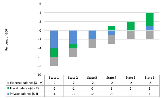
Note also that the government balance equals exactly $-for-$ (as a per cent of GDP) the non-government balance (the sum of the private domestic and external balances). This is also a basic rule derived from the national accounts.
Most countries currently run external deficits. The crisis was marked by households reducing consumption spending growth to try to manage their debt exposure and private investment retreating. The consequence was a major spending gap which pushed fiscal balances into deficit via the automatic stabilisers.
The only way to get income growth going in this context and to allow the private sector surpluses to build was to increase the deficits beyond the impact of the automatic stabilisers. The reality is that this policy change hasn’t delivered large enough fiscal deficits (even with external deficits narrowing). The result has been large negative income adjustments which brought the sectoral balances into equality at significantly lower levels of economic activity.
The following blogs may be of further interest to you:
- Barnaby, better to walk before we run
- Stock-flow consistent macro models
- Norway and sectoral balances
- The OECD is at it again!
Question 2:
Modern Monetary Theory (MMT) makes a crucial distinction between the issuer of the currency and the user of that currency. Unlike a household, which not only has to service its debt obligations over the course of the loan but also has to repay them at the due date, a national government, which issues its own currency can always roll over its “own currency” debt obligations and never has to pay them back.
The answer is False.
As a matter of clarification, note we are discussing debt issued in the currency of issue and not debt denominated in foreign currencies.
First, households do have to service their debts and repay them at some due date or risk default. The other crucial point is that households also have to forego some current consumption, use up savings or run down assets to service their debts and ultimately repay them.
Second, a sovereign government also has to service their debts and repay them at some due date or risk default. There is no difference there. The crucial difference is that unlike a household it does not have to forego any current spending capacity (or privatise public assets) to accomplish these financial transactions.
But the public debt is a legal obligation on government and so is a liability that has to be managed.
Now can it just roll-it over continuously? Well the question was subtle because the government can always keep issuing new debt when the old issues mature. But as the previous debt-issued matures it is paid out as per the terms of the issue.
The other point is that the liability on a sovereign government is legally like all liabilities – enforceable in courts the risk associated with taking that liability on is zero which is very different to the risks attached to taking on private debt.
There is zero financial risk that a holder of a public bond instrument will not be paid principle and interest on time.
The other point to appreciate is that the original holder of the public debt might not be the final holder who is paid out. The market for public debt is the most liquid of all debt markets and trading in public debt instruments of all nations is conducted across all markets each hour of every day.
While I am most familiar with the Australian institutional structure, the following developments are not dissimilar to the way bond issuance (in primary markets) is organised elsewhere. You can access information about this from the Australian Office of Financial Management, which is a Treasury-related public body that manages all public debt issuance in Australia.
It conducts the primary market, which is the institutional machinery via which the government sells debt to the non-government sector.
In a modern monetary system with flexible exchange rates it is clear the government does not have to finance its spending so the fact that governments hang on to primary market issuance is largely ideological – fear of fiscal excesses rather than an intrinsic need.
In this blog – Will we really pay higher interest rates? – I go into this period more fully and show that it was driven by the ideological calls for “fiscal discipline” and the growing influence of the credit rating agencies. Accordingly, all net spending had to be fully placed in the private market $-for-$. A purely voluntary constraint on the government and a waste of time.
A secondary market is where existing financial assets are traded by interested parties. So the financial assets enter the monetary system via the primary market and are then available for trading in the secondary. The same structure applies to private share issues for example.
The company raises funds via the primary issuance process then its shares are traded in secondary markets.
Clearly secondary market trading has no impact at all on the volume of financial assets in the system – it just shuffles the wealth between wealth-holders.
In the context of public debt issuance – the transactions in the primary market are vertical (net financial assets are created or destroyed) and the secondary market transactions are all horizontal (no new financial assets are created).
Please read my blog – Deficit spending 101 – Part 3 – for more information.
Primary issues are conducted via auction tender systems and the Treasury determines the timing of these events in addition to the type and volume of debt to be issued.
The issue is then be put out for tender and the market determines the final price of the bonds issued. Imagine a $A1000 bond is offered at a coupon of 5 per cent, meaning that you would get $A50 dollar per annum until the bond matured at which time you would get $A1000 back.
Imagine that the market wanted a yield of 6 per cent to accommodate risk expectations (see below). So for them the bond is unattractive unless the price is lower than $A1000. So tender system they would put in a purchase bid lower than the $A1000 to ensure they get the 6 per cent return they sought.
The general rule for fixed-income bonds is that when the prices rise, the yield falls and vice versa. Thus, the price of a bond can change in the market place according to interest rate fluctuations.
When interest rates rise, the price of previously issued bonds fall because they are less attractive in comparison to the newly issued bonds, which are offering a higher coupon rates (reflecting current interest rates).
When interest rates fall, the price of older bonds increase, becoming more attractive as newly issued bonds offer a lower coupon rate than the older higher coupon rated bonds.
So for new bond issues the AOFM receives the tenders from the bond market traders. These will be ranked in terms of price (and implied yields desired) and a quantity requested in $ millions. The AOFM (which is really just part of treasury) sometimes sells some bonds to the central bank (RBA) for their open market operations (at the weighted average yield of the final tender).
The AOFM will then issue the bonds in highest price bid order until it raises the revenue it seeks. So the first bidder with the highest price (lowest yield) gets what they want (as long as it doesn’t exhaust the whole tender, which is not likely). Then the second bidder (higher yield) and so on.
In this way, if demand for the tender is low, the final yields will be higher and vice versa. There are a lot of myths peddled in the financial press about this. Rising yields may indicate a rising sense of risk (mostly from future inflation although sovereign credit ratings will influence this). But they may also indicated a recovering economy where people are more confidence investing in commercial paper (for higher returns) and so they demand less of the “risk free” government paper.
So while there is no credit risk attached to holding public debt (that is, the holder knows they will receive the principle and interest that is specified on the issued debt instrument), there is still market risk which is related to movements in interest rates.
For government accounting purposes however the trading of the bonds once issued is of no consequence. They still retain the liability to pay the fixed coupon rate and the face value of the bond at the time of issue (not the market price).
The person/institution that sells the bond before maturity may gain or lose relative to their original purchase price but that is totally outside of the concern of the government.
Its liability is to pay the specified coupon rate at the time of issue and then the whole face value at the time of maturity.
There are complications to the primary sale process – some bonds sell at discounts which imply the coupon value. Further, there are arrangements between treasuries and central banks about the way in which public debt holdings are managed and accounted for. But these nuances do not alter the initial contention – public debt is a liability of the government in just the same way as private debt is a liability for those holders.
The following blogs may be of further interest to you:
Question 3:
Governments concerned with their public debt ratio should encourage growth because the debt ratio falls once economic growth resumes.
The answer is False.
The primary deficit may not fall when economic growth is positive if discretionary policy changes offset the declining net spending as tax revenue increases and welfare payments fall (the automatic stabilisation).
Under current institutional arrangements, governments around the world voluntarily issue debt into the private bond markets to match $-for-$ their net spending flows in each period. A sovereign government within a fiat currency system does not have to issue any debt and could run continuous fiscal deficits (that is, forever) with a zero public debt.
The reason they is covered in the following blogs – On voluntary constraints that undermine public purpose.
The framework for considering this question is provided by the accounting relationship linking the fiscal flows (spending, taxation and interest servicing) with relevant stocks (base money and government bonds).
This framework has been interpreted by the mainstream macroeconomists as constituting an a priori financial constraint on government spending (more on this soon) and by proponents of Modern Monetary Theory (MMT) as an ex post accounting relationship that has to be true in a stock-flow consistent macro model but which carries no particular import other than to measure the changes in stocks between periods.
These changes are also not particularly significant within MMT given that a sovereign government is never revenue constrained because it is the monopoly issuer of the currency.
To understand the difference in viewpoint we might usefully start with the mainstream view.
The way the mainstream macroeconomics textbooks build this narrative is to draw an analogy between the household and the sovereign government and to assert that the microeconomic constraints that are imposed on individual or household choices apply equally without qualification to the government.
The framework for analysing these choices has been called the government fiscal constraint (GBC) in the literature.
The GBC is in fact an accounting statement relating government spending and taxation to stocks of debt and high powered money.
However, the accounting character is downplayed and instead it is presented by mainstream economists as an a priori financial constraint that has to be obeyed. So immediately they shift, without explanation, from an ex post sum that has to be true because it is an accounting identity, to an alleged behavioural constraint on government action.
The GBC is always true ex post but never represents an a priori financial constraint for a sovereign government running a flexible-exchange rate non-convertible currency. That is, the parity between its currency and other currencies floats and the the government does not guarantee to convert the unit of account (the currency) into anything else of value (like gold or silver).
This literature emerged in the 1960s during a period when the neo-classical microeconomists were trying to gain control of the macroeconomic policy agenda by undermining the theoretical validity of the, then, dominant Keynesian macroeconomics.
There was nothing particularly progressive about the macroeconomics of the day which is known as Keynesian although as I explain in this blog – Those bad Keynesians are to blame – that is a bit of a misnomer.
Anyway, just as an individual or a household is conceived in orthodox microeconomic theory to maximise utility (real income) subject to their fiscal constraints, this emerging approach also constructed the government as being constrained by a “financing” constraint.
Accordingly, they developed an analytical framework whereby the fiscal deficits had stock implications – this is the so-called ‘Government Budget Constraint’, which is more accurately just a ‘Government Fiscal Accounting Relation’.
So within this model, taxes are conceived as providing the funds to the government to allow it to spend.
Further, this approach asserts that any excess in government spending over taxation receipts then has to be “financed” in two ways: (a) by borrowing from the public; and (b) by printing money.
You can see that the approach is a ‘gold standard’ approach where the quantity of “money” in circulation is proportional (via a fixed exchange price) to the stock of gold that a nation holds at any point in time. So if the government wants to spend more it has to take money off the non-government sector either via taxation of bond-issuance.
However, in a fiat currency system, the mainstream analogy between the household and the government is flawed at the most elemental level. The household must work out the financing before it can spend. The household cannot spend first. The government can spend first and ultimately does not have to worry about financing such expenditure.
From a policy perspective, they believed (via the flawed Quantity Theory of Money) that ‘printing money’ would be inflationary (even though governments do not spend by printing money anyway.
So they recommended that deficits be covered by debt-issuance, which they then claimed would increase interest rates by increasing demand for scarce savings and crowd out private investment.
All sorts of variations on this nonsense has appeared ranging from the moderate Keynesians (and some Post Keynesians) who claim the ‘financial crowding out’ (via interest rate increases) is moderate to the extreme conservatives who say it is 100 per cent (that is, no output increase accompanies government spending).
So the Government Fiscal Accounting Relation, which the mainstream macroeconomics framework calls the ‘Government Budget Constraint’ just tells us what will happen in accounting terms when government spending and taxation changes, assuming governments match their deficits with debt issuance.
In accounting terms, it just says that the Fiscal deficit in year t is equal to the change in government debt (ΔB) over year t plus the change in central bank (base) money (ΔH) over year t.
If we think of this in real terms (rather than monetary terms), the mathematical expression of this is written as:
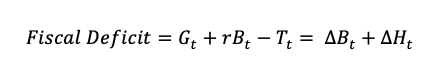
which you can read in English as saying that the overall Fiscal deficit is equal to Government spending (G) Government interest payments (rBt-1) – Tax receipts (T).
However, this is merely an accounting statement. It has to be true if things have been added and subtracted properly in accounting for the dealings between the government and non-government sectors.
In mainstream macroeconomics, the accounting relationship is erroneously held out to be a financing constraint on government spending.
In mainstream economics, money creation is erroneously depicted as the government asking the central bank to buy treasury bonds which the central bank in return then prints money.
The government then spends this money.
This is called debt monetisation and we have shown in the Deficits 101 series how this conception is incorrect.
Anyway, the mainstream claims that if the government is willing to increase the money growth rate it can finance a growing deficit but also inflation because there will be too much money chasing too few goods!
But an economy constrained by deficient demand (defined as demand below the full employment level) responds to a nominal impulse by expanding real output not prices.
The claim that inflation is inevitable if ΔH > 0 (the so-called ‘printing money’ option) leads mainstream economists to recommend that governments use debt issuance to ‘finance’ their deficits. But then they scream that this will merely require higher future taxes. Why should taxes have to be increased?
Well the textbooks are full of elaborate models of debt pay-back, debt stabilisation etc which all ‘prove’ (not!) that the legacy of past deficits is higher debt and to stabilise the debt, the government must eliminate the deficit which means it must then run a primary surplus equal to interest payments on the existing debt.
Nothing is included about the swings and roundabouts provided by the automatic stabilisers as the results of the deficits stimulate private activity and welfare spending drops and tax revenue rises automatically in line with the increased economic growth. Most orthodox models are based on the assumption of full employment anyway, which makes them nonsensical depictions of the real world.
More sophisticated mainstream analyses focus on the ratio of debt to GDP rather than the level of debt per se. They come up with the following equation – nothing that they now disregard the obvious opportunity presented to the government via ΔH. So in the following model all net public spending is covered by new debt-issuance (even though in a fiat currency system no such financing is required).
Accordingly, the change in the public debt ratio is:
![]()
The change in the debt ratio is the sum of two terms on the right-hand side: (a) the difference between the real interest rate (r) and the GDP growth rate (g) times the initial debt ratio; and (b) the ratio of the primary deficit (G-T) to GDP.
A growing economy can absorb more debt and keep the debt ratio constant. For example, if the primary deficit is zero, debt increases at a rate r but the debt ratio increases at r – g.
So a change in the change in the debt ratio is the sum of two terms on the right-hand side: (a) the difference between the real interest rate (r) and the GDP growth rate (g) times the initial debt ratio; and (b) the ratio of the primary deficit (G-T) to GDP.
As we noted a growing economy can absorb more debt and keep the debt ratio constant. For example, if the primary deficit is zero, debt increases at a rate r but the debt ratio increases at r – g.
Consider the following table which simulates two different scenarios.
Case A: where the government matches the primary fiscal deficit with debt-issuance.
Case B: where the government does not issue debt in any subsequent year.
The economy has a real interest rate of zero and a steadily increasing annual GDP growth rate across 10 years.
The initial public debt ratio is 100 per cent (well over the level Reinhart and Rogoff claim is the point of no return where insolvency is pending).
The primary fiscal deficit is also simulated to be 5 per cent of GDP then reduces as the GDP growth induce the automatic stabilisers.
It then reaches a steady 2 per cent per annum which might be sufficient to support the saving intentions of the non-government sector while still promoting steady economic growth.
Under Case A, even with a continuous primary fiscal deficit, the public debt ratio declines steadily once real GDP exceeds it, and would continue to do so as the growth continued.
In Case B, the public debt ratio drops very quickly as no new debt is issued.
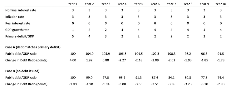
However, should the real interest rate exceed the economic growth rate, then unless the primary fiscal balance offsets the rising interest payments as percent of GDP, then the public debt ratio will rise.
The only concern I would have in this situation does not relate to the rising ratio. Focusing on the cause should be the policy concern.
If the real economy is faltering because interest rates are too high or more likely because the primary fiscal deficit is too low then the rising public debt ratio is just telling us that the central bank should drop interest rates or the treasury should increase the discretionary component of the fiscal balance.
In general though, the public debt ratio is a relatively uninteresting macroeconomic figure and should be disregarded. If the government is intent on promoting growth, then the primary deficit ratio and the public debt ratio will take care of themselves.
You may be interested in reading these blogs which have further information on this topic:
- On voluntary constraints that undermine public purpose
- Deficits 101 series
- Questions and answers 1
- Will we really pay higher taxes?
- Will we really pay higher interest rates?
That is enough for today!
(c) Copyright 2018 William Mitchell. All Rights Reserved.
So what’s the thing about the comments gone Bill? Don’t want people linking to your own posts? What did I do wrong this time? Was the discussion off topic for MMT? And what was wrong with me telling Gia they might like to read your blog “The case against free trade part 4”? Actually it might be- “A surplus of trade discussions” – I forget which one I recommended to Simon and which to Gia. Either way, they are both good to read. Here are the links again and you can delete them and my comments as you see fit. Not that I appreciate that in any way. But it is your blog after all.
https://billmitchell.org/blog/?p=34860 “The case against free trade- part 4”
https://billmitchell.org/blog/?p=39420 “A surplus of trade discussions”
Dear Jerry Brown (at 2018/11/04 at 9:21 am)
Sorry Jerry. I deleted a few comments this morning because they were pointing to an external commentary that I didn’t wish to link to. I inadvertently mistook your comment for one of that series.
I also apologise to the other participants who took their time to make those (deleted) comments. I value your time as much as I value my own.
The problem was that the material linked to was not offered in good faith. It is part of a series of attacks on Modern Monetary Theory (MMT) and myself personally that pretend to expose deficiencies in our work but ignore many years of work on the topics covered.
I have no intention of privileging such material. If there is commentary that is in good faith and reflects a knowledge of our work and thinks we are mistaken then I will respond.
But dishonest and personal attacks are just fake posturing from attention seekers and they deserve no oxygen at all.
I do not like censorship but my blog and our work is about advancing knowledge not scuttlebutt (fake claims) and personal enmity.
best wishes
bill
Thank you for the explanation Bill. I understand.
But maybe you should have more confidence in your ability to educate and the strength of your arguments and analysis. And on the ability of your readers to utilize what you have taught.
On the other hand, going from my success at these quizzes, maybe you shouldn’t get too overly optimistic either. About 80% optimistic would be about right, if that makes any sense 🙂
Thanks for the education. And thank you for the quizzes and the blog.
As soon as the messages disappeared it “clicked”.Well understood Bill, well understood.
‘On the other hand, going from my success at these quizzes, maybe you shouldn’t get too overly optimistic either. About 80% optimistic would be about right, if that makes any sense :)’
Having read Bill’s posts for a few years whilst climbing the steep learning curve that confronts anyone coming from a background of zero knowledge, I’m often shocked at how little I recall and how many times I have to re-read the same material. Could be that my cognitive skills are poor or that it is partly to do with not studying the material in a formal setting (academically) where one has more of a framework to support the learning. Maybe the MMT University idea that Bill is working on would help with that. Although I think the subject favours people with good skills at combinatorial thinking so that mathematicians and engineer types, who have to hold complex patterns of relationships in their heads, fair better. I’ve often thought of giving up and accepting I’m just not ‘up to it’ but then I realise that I’ve probably learnt more than I think from reading Bill and other MMT economists even if I haven’t got a good command of it.
Don’t give up Simon- the quizzes are designed to be challenging. And they are. That’s why I love them. If you are reading the blog you are learning this stuff. I like to think of it as now I have a BS bell that goes off when I’m listening to some politician on the news or reading some other economist’s statements about what we need to do. Beforehand, I might have thought that what they said seemed reasonable- now that bell goes off and its like ‘no- that’s not necessarily true’, or ‘no- that’s completely wrong’. Its amazing how often that bell goes off now. I’m going to need ear plugs or something.