Here are the answers with discussion for this Weekend’s Quiz. The information provided should help you work out why you missed a question or three! If you haven’t already done the Quiz from yesterday then have a go at it before you read the answers. I hope this helps you develop an understanding of Modern…
The Weekend Quiz – January 19-20, 2019 – answers and discussion
Here are the answers with discussion for this Weekend’s Quiz. The information provided should help you work out why you missed a question or three! If you haven’t already done the Quiz from yesterday then have a go at it before you read the answers. I hope this helps you develop an understanding of Modern Monetary Theory (MMT) and its application to macroeconomic thinking. Comments as usual welcome, especially if I have made an error.
Question 1:
If economy-wide average nominal wages fail to keep pace with the inflation rate then it means the profit share in GDP is rising.
The answer is False.
We also have to consider productivity movements.
The wage share in nominal GDP is expressed as the total wage bill as a percentage of nominal GDP. Economists differentiate between nominal GDP ($GDP), which is total output produced at market prices and real GDP (GDP), which is the actual physical equivalent of the nominal GDP. We will come back to that distinction soon.
To compute the wage share we need to consider total labour costs in production and the flow of production ($GDP) each period.
Employment (L) is a stock and is measured in persons (averaged over some period like a month or a quarter or a year.
The wage bill is a flow and is the product of total employment (L) and the average nominal wage (w) prevailing at any point in time. Stocks (L) become flows if it is multiplied by a flow variable (W). So the wage bill is the total labour costs in production per period.
So the wage bill = W.L
The wage share is just the total labour costs expressed as a proportion of $GDP – (W.L)/$GDP in nominal terms, usually expressed as a percentage. We can actually break this down further.
Labour productivity (LP) is the units of real GDP per person employed per period. Using the symbols already defined this can be written as:
LP = GDP/L
so it tells us what real output (GDP) each labour unit that is added to production produces on average.
We can also define another term that is regularly used in the media – the real wage – which is the purchasing power equivalent on the nominal wage that workers get paid each period. To compute the real wage we need to consider two variables: (a) the nominal wage (W) and the aggregate price level (P).
We might consider the aggregate price level to be measured by the consumer price index (CPI) although there are huge debates about that.
Now the nominal wage (W) – that is paid by employers to workers is determined in the labour market – by the contract of employment between the worker and the employer.
The price level (P) is determined in the goods market – by the interaction of total supply of output and aggregate demand for that output although there are complex models of firm price setting that use cost-plus mark-up formulas with demand just determining volume sold.
The inflation rate is just the continuous growth in the price level (P). A once-off adjustment in the price level is not considered by economists to constitute inflation.
So the real wage (w) tells us what volume of real goods and services the nominal wage (W) will be able to command and is obviously influenced by the level of W and the price level.
For a given W, the lower is P the greater the purchasing power of the nominal wage and so the higher is the real wage (w).
We write the real wage (w) as W/P. So if W = 10 and P = 1, then the real wage (w) = 10 meaning that the current wage will buy 10 units of real output. If P rose to 2 then w = 5, meaning the real wage was now cut by one-half.
Nominal GDP ($GDP) can be written as P.GDP, where the P values the real physical output.
Now if you put of these concepts together you get an interesting framework. To help you follow the logic here are the terms developed and be careful not to confuse $GDP (nominal) with GDP (real):
- Wage share = (W.L)/$GDP
- Nominal GDP: $GDP = P.GDP
- Labour productivity: LP = GDP/L
- Real wage: w = W/P
By substituting the expression for Nominal GDP into the wage share measure we get:
Wage share = (W.L)/P.GDP
In this area of economics, we often look for alternative way to write this expression – it maintains the equivalence (that is, obeys all the rules of algebra) but presents the expression (in this case the wage share) in a different “view”.
So we can write as an equivalent:
Wage share = (W/P).(L/GDP)
Now if you note that (L/GDP) is the inverse (reciprocal) of the labour productivity term (GDP/L). We can use another rule of algebra (reversing the invert and multiply rule) to rewrite this expression again in a more interpretable fashion.
So an equivalent but more convenient measure of the wage share is:
Wage share = (W/P)/(GDP/L) – that is, the real wage (W/P) divided by labour productivity (GDP/L).
I won’t show this but I could also express this in growth terms such that if the growth in the real wage equals labour productivity growth the wage share is constant. The algebra is simple but we have done enough of that already.
That journey might have seemed difficult to non-economists (or those not well-versed in algebra) but it produces a very easy to understand formula for the wage share.
Two other points to note.
The wage share is also equivalent to the real unit labour cost (RULC) measures that Treasuries and central banks use to describe trends in costs within the economy.
Please read my blog – Saturday Quiz – May 15, 2010 – answers and discussion – for more discussion on this point.
Now it becomes obvious that if the nominal wage (W) and the price level (P) are growing at the pace the real wage is constant. And if the real wage is growing at the same rate as labour productivity, then both terms in the wage share ratio are equal and so the wage share is constant.
However, if the real wage is falling we cannot conclude that the wage share is also falling. Given the nature of ratios, if the numerator (in this case, the real wage) is falling but not by as much as the denominator (in this case, labour productivity) then the overall ratio can actually be rising.
The following blog posts may be of further interest to you:
- The origins of the economic crisis
- The fiscal stimulus worked but was captured by profits
- When will the workers wake up?
Question 2:
Assume that a national is continuously running an external deficit of 2 per cent of GDP. In this economy, if the private domestic sector successfully saves overall, we would always find:
(a) Cannot tell because we don’t know the scale of the private domestic sector saving as a % of GDP.
(b) A fiscal surplus.
(c) A fiscal deficit.
The answer is Option (c) – A fiscal deficit..
This question requires an understanding of the sectoral balances that can be derived from the National Accounts. But it also requires some understanding of the behavioural relationships within and between these sectors which generate the outcomes that are captured in the National Accounts and summarised by the sectoral balances.
To refresh your memory the balances are derived as follows. The basic income-expenditure model in macroeconomics can be viewed in (at least) two ways: (a) from the perspective of the sources of spending; and (b) from the perspective of the uses of the income produced. Bringing these two perspectives (of the same thing) together generates the sectoral balances.
From the sources perspective we write:
(1) GDP = C + I + G + (X – M)
which says that total national income (GDP) is the sum of total final consumption spending (C), total private investment (I), total government spending (G) and net exports (X – M).
Expression (1) tells us that total income in the economy per period will be exactly equal to total spending from all sources of expenditure.
We also have to acknowledge that financial balances of the sectors are impacted by net government taxes (T) which includes all tax revenue minus total transfer and interest payments (the latter are not counted independently in the expenditure Expression (1)).
Further, as noted above the trade account is only one aspect of the financial flows between the domestic economy and the external sector. we have to include net external income flows (FNI).
Adding in the net external income flows (FNI) to Expression (2) for GDP we get the familiar gross national product or gross national income measure (GNP):
(2) GNP = C + I + G + (X – M) + FNI
To render this approach into the sectoral balances form, we subtract total net taxes (T) from both sides of Expression (3) to get:
(3) GNP – T = C + I + G + (X – M) + FNI – T
Now we can collect the terms by arranging them according to the three sectoral balances:
(4) (GNP – C – T) – I = (G – T) + (X – M + FNI)
The the terms in Expression (4) are relatively easy to understand now.
The term (GNP – C – T) represents total income less the amount consumed less the amount paid to government in taxes (taking into account transfers coming the other way). In other words, it represents private domestic saving.
The left-hand side of Equation (4), (GNP – C – T) – I, thus is the overall saving of the private domestic sector, which is distinct from total household saving denoted by the term (GNP – C – T).
In other words, the left-hand side of Equation (4) is the private domestic financial balance and if it is positive then the sector is spending less than its total income and if it is negative the sector is spending more than it total income.
The term (G – T) is the government financial balance and is in deficit if government spending (G) is greater than government tax revenue minus transfers (T), and in surplus if the balance is negative.
Finally, the other right-hand side term (X – M + FNI) is the external financial balance, commonly known as the current account balance (CAD). It is in surplus if positive and deficit if negative.
In English we could say that:
The private financial balance equals the sum of the government financial balance plus the current account balance.
We can re-write Expression (6) in this way to get the sectoral balances equation:
(5) (S – I) = (G – T) + CAB
which is interpreted as meaning that government sector deficits (G – T > 0) and current account surpluses (CAB > 0) generate national income and net financial assets for the private domestic sector.
Conversely, government surpluses (G – T < 0) and current account deficits (CAB < 0) reduce national income and undermine the capacity of the private domestic sector to add financial assets.
Expression (5) can also be written as:
(6) [(S – I) – CAB] = (G – T)
where the term on the left-hand side [(S – I) – CAB] is the non-government sector financial balance and is of equal and opposite sign to the government financial balance.
This is the familiar MMT statement that a government sector deficit (surplus) is equal dollar-for-dollar to the non-government sector surplus (deficit).
The sectoral balances equation says that total private savings (S) minus private investment (I) has to equal the public deficit (spending, G minus taxes, T) plus net exports (exports (X) minus imports (M)) plus net income transfers.
All these relationships (equations) hold as a matter of accounting and not matters of opinion.
So what economic behaviour might lead to the outcome specified in the question?
If the nation is running an external deficit it means that the contribution to aggregate demand from the external sector is negative – that is net drain of spending – dragging output down. The reference to the specific 2 per cent of GDP figure was to place doubt in your mind. In fact, it doesn’t matter how large or small the external deficit is for this question.
Assume, now that the private domestic sector (households and firms) seeks to increase its overall saving ratio (the gap between overall private domestic spending and the income it receives as a proportion of its total income) and is successful in doing so.
Consistent with this aspiration, households may cut back on consumption spending and save more out of disposable income. Firms may also reduce their spending (investment).
The immediate impact is that aggregate demand will fall and inventories will start to increase beyond the desired level of the firms.
Firms will soon react to the increased inventory holding costs and will start to cut back production.
How quickly this happens depends on a number of factors including the pace and magnitude of the initial demand contraction. But if the households persist in trying to save more and consumption continues to lag, then soon enough the economy starts to contract – output, employment and income all fall.
The initial contraction in consumption multiplies through the expenditure system as workers who are laid off also lose income and their spending declines. This leads to further contractions.
The declining income leads to a number of consequences. Net exports improve as imports fall (less income) but the question clearly assumes that the external sector remains in deficit. Total saving actually starts to decline as income falls as does induced consumption.
So the initial discretionary decline in consumption is supplemented by the induced consumption falls driven by the multiplier process.
The decline in income then stifles firms’ investment plans – they become pessimistic of the chances of realising the output derived from augmented capacity and so aggregate demand plunges further. Both these effects push the private domestic balance further towards and eventually into surplus
With the economy in decline, tax revenue falls and welfare payments rise which push the public fiscal balance towards and eventually into deficit via the automatic stabilisers.
If the private sector persists in trying to increase its overall saving ratio then the contracting income will clearly push the fiscal balance into deficit or into greater deficit (depending of the starting position).
The undeniable result is that if there is an external deficit and the private domestic sector saves overall (a surplus) then there will always be a fiscal deficit.
The higher the overall private saving, the larger will be the fiscal deficit.
The following blogs may be of further interest to you:
- Barnaby, better to walk before we run
- Stock-flow consistent macro models
- Norway and sectoral balances
- The OECD is at it again!
Question 3:
Assume that the inflation and nominal interest rates both zero and constant. Consider a country with a public debt to GDP ratio of 100 per cent, which the mainstream economists consider to be dangerously high. The mainstream prescription is to run primary fiscal surpluses to stabilise and then reduce the debt ratio. Under the circumstances given, this strategy will only work if there is positive real GDP growth.
The answer is False.
First, some background theory and conceptual development.
While Modern Monetary Theory (MMT) places no particular importance in the public debt to GDP ratio for a sovereign government, given that insolvency is not an issue, the mainstream debate is dominated by the concept.
The unnecessary practice employed by fiat currency-issuing governments of issuing public debt $-for-$ to match public net spending (deficits) ensures that the debt levels will always rise when there are fiscal deficits.
But the rising debt levels do not necessarily have to rise at the same rate as GDP grows. The question is about the debt ratio not the level of debt per se.
Rising deficits often are associated with declining economic activity (especially if there is no evidence of accelerating inflation) which suggests that the debt/GDP ratio may be rising because the denominator is also likely to be falling or rising below trend.
Further, historical experience tells us that when economic growth resumes after a major recession, during which the public debt ratio can rise sharply, the latter always declines again.
It is this endogenous nature of the ratio that suggests it is far more important to focus on the underlying economic problems which the public debt ratio just mirrors.
Mainstream economics starts with the flawed analogy between the household and the sovereign government such that any excess in government spending over taxation receipts has to be “financed” in two ways: (a) by borrowing from the public; and/or (b) by “printing money”.
Neither characterisation is remotely representative of what happens in the real world in terms of the operations that define transactions between the government and non-government sector.
Further, the basic analogy is flawed at its most elemental level. The household must work out the financing before it can spend. The household cannot spend first. The government can spend first and ultimately does not have to worry about financing such expenditure.
However, in mainstream theory, the framework for analysing these so-called ‘financing’ choices is called the government budget constraint (GBC).
The GBC is written as:
![]()
which you can read in English as saying that fiscal deficit in any year (t) = Government spending (G) + Government interest payments (rBt-1) – Tax receipts (T) must equal (be “financed” by) a change in Bonds ((ΔB)) and/or a change in high powered money ((ΔH)). The triangle sign (delta) is just shorthand for the change in a variable. The subscript t means the current period and t-1 is the previous period.
From an MMT perspective, this equation is just an ex post accounting identity that has to be true by definition and has no real economic importance.
In a stock-flow consistent macroeconomics, this statement will always hold. That is, it has to be true if all the transactions between the government and non-government sector have been correctly added and subtracted.
MMT tells us that there is no ‘funding’ constraint on government deficits.
But for the mainstream economist, the equation represents an ex ante (before the fact) financial constraint that the government is bound by.
The difference between these two conceptions is very significant and the second (mainstream) interpretation cannot be correct if governments issue fiat currency (unless they place voluntary constraints on themselves and act as if it is a financial constraint).
Further, in mainstream economics, money creation is erroneously depicted as the government asking the central bank to buy treasury bonds which the central bank in return then prints money. The government then spends this money.
This is called debt monetisation and you can find out why this is typically not a viable option for a central bank by reading the Deficits 101 suite – Deficit spending 101 – Part 1 – Deficit spending 101 – Part 2 – Deficit spending 101 – Part 3.
Further, the mainstream theory claims that if governments increase the money growth rate (they erroneously call this “printing money”) the extra spending will cause accelerating inflation because there will be “too much money chasing too few goods”!
Of-course, we know that proposition to be generally preposterous because economies that are constrained by deficient demand (defined as demand below the full employment level) respond to nominal demand increases by expanding real output rather than prices. There is an extensive literature pointing to this result.
So when governments are expanding deficits to offset a collapse in private spending, there is typically plenty of spare capacity available to ensure output rather than inflation increases.
Nothwithstanding the reality, the mainstream economists thus eschew ‘monetary’ funding options, and argue that as a better (but still poor) solution, governments should use debt issuance to “finance” their deficits.
Thy also claim this is a poor option because in the short-term it is alleged to increase interest rates and in the longer-term is results in higher future tax rates because the debt has to be “paid back”.
Neither proposition bears scrutiny – you can read these blog posts – Will we really pay higher taxes? and Will we really pay higher interest rates? – for further discussion on these points.
Now to the question.
A primary fiscal balance is the difference between government spending (excluding interest rate servicing) and taxation revenue.
The standard mainstream framework, which even the so-called progressives (deficit-doves) use, focuses on the ratio of debt to GDP rather than the level of debt per se.
The following equation captures the approach:
![]()
So the change in the debt ratio is equal to the sum of two terms on the right-hand side:
1. The difference between the real interest rate (r) and the GDP growth rate (g) times the initial debt ratio; and
2. The ratio of the primary deficit (G-T) to GDP.
The real interest rate is the difference between the nominal interest rate and the inflation rate.
This standard mainstream framework is used to highlight the dangers of running deficits. But even progressives (not me) use it in a perverse way to justify deficits in a downturn balanced by surpluses in the upturn.
Many mainstream economists and a fair number of so-called progressive economists say that governments should as some point in the business cycle run primary surpluses (taxation revenue in excess of non-interest government spending) to start reducing the debt ratio back to “safe” territory.
Almost all the media commentators that you read on this topic take it for granted that the only way to reduce the public debt ratio is to run primary surpluses. That is what the whole “credible exit strategy” rhetoric is about and what is driving the austerity push around the world at present.
The standard formula above can easily demonstrate that a nation running a primary deficit can reduce its public debt ratio over time.
So it is clear that the public debt ratio can fall even if there is an on-going fiscal deficit if the real GDP growth rate is strong enough. This is win-win way to reduce the public debt ratio.
But the question is analysing the situation where the government is desiring to run primary fiscal surpluses.
Consider the following Table which captures the variations possible in the question.
In Year 1, the B/Y(-1) = 1 (that is, the public debt ratio at the start of the period is 100 per cent). The (-1) just signals the value inherited in the current period.
We have already assumed that the inflation rate and the nominal interest rate are constant and zero, which means that the real interest rate is also zero and constant. So the r term in the model is 0 throughout our stylised simulation.
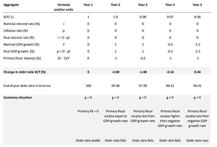
In Year 1, there is zero real GDP growth and the Primary fiscal balance is also zero. Under these circumstances, the debt ratio is stable.
Now in Year 2, the fiscal austerity program begins and assume for the sake of discussion that it doesn’t dent real GDP growth.
In reality, a major fiscal contraction is likely to push real GDP growth into the negative (that is, promote a recession).
But for the sake of the logic we assume that nominal GDP growth is 1 per cent in Year 2, which means that real GDP growth is also 1 per cent given that all the nominal growth is real (zero inflation).
We assume that the government succeeds in pushing the Primary fiscal surplus to 1 per cent of GDP. This is the mainstream nirvana – the public debt ratio falls by 2 per cent as a consequence.
In Year 3, we see that the Primary fiscal surplus remains positive (0.5 per cent of GDP) but is now below the positive real GDP growth rate.
In this case the public debt ratio still falls because the GDP growth rate is deflating the denominator of the public debt ratio while the numerator is falling due to the primary fiscal surplus.
In Year 4, real GDP growth contracts (0.5 per cent) and the Primary fiscal surplus remains positive (1 per cent of GDP). In this case the public debt ratio still fall which makes the proposition in the question false.
This result occurs because the numerator is falling faster than the falling denominator.
So if you have zero real interest rates, then even in a recession, the public debt ratio can still fall and the government run a fiscal surplus as long as Primary surplus is greater in absolute value to the negative real GDP growth rate.
Of-course, this logic is just arithmetic based on the relationship between the flows and stocks involved. In reality, it would be hard for the government to run a primary surplus under these conditions given the automatic stabilisers would be undermining that aim.
In Year 5, the real GDP growth rate is negative 1.5 per cent and the Primary fiscal surplus remains positive at 1 per cent of GDP. In this case the public debt ratio rises.
This would be the typical situation.
The best way to reduce the public debt ratio is to stop issuing debt. A sovereign government doesn’t have to issue debt if the central bank is happy to keep its target interest rate at zero or pay interest on excess reserves.
The discussion also demonstrates why tightening monetary policy makes it harder for the government to reduce the public debt ratio – which, of-course, is one of the more subtle mainstream ways to force the government to run surpluses.
The following blog may be of further interest to you:
That is enough for today!
(c) Copyright 2019 William Mitchell. All Rights Reserved.
On another site I read one of the poster posted this. Could someone tell me why he is wrong where I tried to bold it.
.
“MMT isn’t new, and precisely because it isn’t new, we can also see whether it’s predictive or not: And guess what? It isn’t. In a sense, it’s not a monetary theory at all: It’s a theory about fiscal policy (It’s OK to increase deficits a whole lot), but all the talks about money destruction, as if macroeconomics what really accounting, just doesn’t make sense. [b]The whole ‘lower government deficits mean higher private sector deficits’, doesn’t really work in reality.[/b]
.
That of course doesn’t mean that the US can’t borrow more than it does, just that their reasoning for this stands on nothing, just like the people that want to lower taxes no matter what because it will always increase revenue.”
Dear Steve_American (at 2019/01/20 at 4:21 pm)
Better to ignore this type of opinion.
This sort of arrogance (which is disguising ignorance) is becoming common now as more and more people are realising their ideas are looking flaky.
Engaging with them gives their defunct views and arrogance ill-deserved oxygen. They will not change through discussion and soon turn to personal abuse.
I cannot see the point of slugging it out on the Internet with strangers who hold views like this.
It is better to let the current MMT wave flow straight past them and leave them stranded with their irrelevance.
best wishes
bill
Hi Bill!
Your words have been used to respond to me whenever I make an argument for MMT in other forums 🙂
However, I agree that one has to choose the battles worth fighting wisely, if one is to win the war.
@ Steve American
Should you choose to ignore Bill’s wise advice, you can point to the following:
Predictive capability: most MMT economists actually foresaw the GFC and the “difficulties” of the common currency in Europe and refused to believe the proclamation of tthe “Great Moderation”. Also you could point at their refusal to acknowledge the impending doom to befall Japan because of their public debt/deficit while in fact the mainstream keeps “adjusting” their predictions and rescheduling that crisis for a later time. Also, if that poster goes by predictive capability, surely he is not in favor of the neoliberal mainstream either, is he?
“The whole ‘lower government deficits mean higher private sector deficits’, doesn’t really work in reality.”
That guy has either never heard of the current account balance (CAB), in which case his ignorance about MMT should prompt you to ignore him (or try to educate him), or he is deliberately leaving it out in order to make a point, in which case he is being intellectually dishonest.
I would probably follow Bill’s advice, but if you don’t: give him hell!
Hermann, I’m not going to reply to him.
.
The ‘lower government deficits mean higher private sector deficits’ sentence seems sort of like a double negative and so is hard to understand.
If i changed it to ‘lower government deficits mean lower private sector surpluses’, wouldn’t that be easier to understand? And more likely to be true in most cases?
.
But, thanks for your reply.
@ Steve
“And more likely to be true in most cases?”
I think that would only be the case if you disregard the CAB, i.e. in a “closed economy”. I’ll venture into the (simplified) sectoral balances to make my point and hope somebody swiftly corrects and reprimends me should I make a mistake:
Sectoral balance in open economy (from eq. 6 further up in this post):
(S – I) = (G – T) + CAB
“which is interpreted as meaning that government sector deficits (G – T > 0) and current account surpluses (CAB > 0) generate national income and net financial assets for the private domestic sector.”
So, in the case of a closed economy we disregard the CAB, which yields:
(S – I) = (G- T)
For the private sector to see a surplus, (S – I) > 0, the government needs to spend more than it taxes so G – T > 0 as well.
Since we are discussing educating unrelenting neoliberals, I would welcome any suggestions for countering the neo-mercantilistic approach that all countries can achieve balanced budgets if they only export more and import less (nevermind there is little reason to force a balanced budget to begin with). The logical step, that not all countries can export more than they import at the same time is often countered by the moralistic view that exporting countries are thriftier and more disciplined than those “lazy southerners”. This thinly-veiled discrimination is used to justify the “Japan anomally” as well and is hard to counter, because it’s pure gut and little brain.
Cheers!