The Weekend Quiz – March 9-10, 2019 – answers and discussion

Here are the answers with discussion for this Weekend’s Quiz. The information provided should help you work out why you missed a question or three! If you haven’t already done the Quiz from yesterday then have a go at it before you read the answers. I hope this helps you develop an understanding of modern monetary theory (MMT) and its application to macroeconomic thinking. Comments as usual welcome, especially if I have made an error.

Question 1:

A central bank can pay any rate on excess reserves to the commercial banks that it chooses independent of its other monetary policy settings.

The answer is False.

The facts are as follows. First, central banks will always provide enough reserve balances to the commercial banks at a price it sets using a combination of overdraft/discounting facilities and open market operations.

Second, if the central bank didn’t provide the reserves necessary to match the growth in deposits in the commercial banking system then the payments system could grind to a halt and there would be significant hikes in the interbank rate of interest and a wedge between it and the policy (target) rate – meaning the central bank’s policy stance becomes compromised.

Third, any reserve requirements within this context while legally enforceable (via fines etc) do not constrain the commercial bank credit creation capacity.

Central bank reserves (the accounts the commercial banks keep with the central bank) are not used to make loans.

They only function to facilitate the payments system (apart from satisfying any reserve requirements).

Fourth, banks make loans to credit-worthy borrowers and these loans create deposits. If the commercial bank in question is unable to get the reserves necessary to meet the requirements from other sources (other banks) then the central bank has to provide them.

But the process of gaining the necessary reserves is a separate and subsequent bank operation to the deposit creation (via the loan).

Fifth, if there were too many reserves in the system (relative to the banks’ desired levels to facilitate the payments system and the required reserves then competition in the interbank (overnight) market would drive the interest rate down.

This competition would be driven by banks holding surplus reserves (to their requirements) trying to lend them overnight.

The opposite would happen if there were too few reserves supplied by the central bank. Then the chase for overnight funds would drive rates up.

In both cases the central bank would lose control of its current policy rate as the divergence between it and the interbank rate widened.

This divergence can snake between the rate that the central bank pays on excess reserves (this rate varies between countries and overtime but before the crisis was zero in Japan and the US) and the penalty rate that the central bank seeks for providing the commercial banks access to the overdraft/discount facility.

So the aim of the central bank is to issue just as many reserves that are required for the law and the banks’ own desires.

Now the question asks whether the central bank can set whatever penalty rate that it charges for providing reserves to the banks that it likes.

The answer is no because the target rate (the short-term policy rate and the support or penalty rate are closely linked – the former constraining the latter).

The wider the spread between these rates the more difficult is it for the central bank to ensure the quantity of reserves is appropriate for maintaining its target (policy) rate.

Where this spread is narrow, central banks “hit” their target rate each day more precisely than when the spread is wider.

So if the central bank really wanted to put the screws on commercial bank lending via increasing the penalty rate, it would have to be prepared to lift its target rate in close correspondence.

In other words, its monetary policy stance becomes beholden to the discount window settings.

The best answer was False because the central bank cannot operate with wide divergences between the penalty rate and the target rate and it is likely that the former would have to rise significantly to choke private bank credit creation.

You might like to read this blog for further information:

• US federal reserve governor is part of the problem
• Building bank reserves will not expand credit
• Building bank reserves is not inflationary

Question 2:

Only one of the following propositions is possible (with all balances expressed as a per cent of GDP):

• A nation can export less than the sum of imports, net factor income (such as interest and dividends) and net transfer payments (such as foreign aid) and run a government surplus of equal proportion to GDP, while the private domestic sector is spending less than they are earning.
• A nation can export less than the sum of imports, net factor income (such as interest and dividends) and net transfer payments (such as foreign aid) and run a government sector surplus of equal proportion to GDP, while the private domestic sector is spending more than they are earning.
• A nation can export less than the sum of imports, net factor income (such as interest and dividends) and net transfer payments (such as foreign aid) and run a government sector surplus that is larger, while the private domestic sector is spending less than they are earning.
• None of the above are possible as they all defy the sectoral balances accounting identity.

The correct answer is the Option (b) – “A nation can run a current account deficit accompanied by a government sector surplus of equal proportion to GDP, while the private domestic sector is spending more than they are earning”.

Note that the the current account is equal to the trade balance plus invisibles. The trade balance is exports minus imports and the invisibles are equal to the sum of net factor income (such as interest and dividends) and net transfer payments (such as foreign aid). So the question is asking about a current account deficit.

This is a question about the sectoral balances – the government fiscal balance, the external balance and the private domestic balance – that have to always add to zero because they are derived as an accounting identity from the national accounts.

To refresh your memory the balances are derived as follows. The basic income-expenditure model in macroeconomics can be viewed in (at least) two ways: (a) from the perspective of the sources of spending; and (b) from the perspective of the uses of the income produced. Bringing these two perspectives (of the same thing) together generates the sectoral balances.

From the sources perspective we write:

(1) GDP = C + I + G + (X – M)

which says that total national income (GDP) is the sum of total final consumption spending (C), total private investment (I), total government spending (G) and net exports (X – M).

Expression (1) tells us that total income in the economy per period will be exactly equal to total spending from all sources of expenditure.

We also have to acknowledge that financial balances of the sectors are impacted by net government taxes (T) which includes all tax revenue minus total transfer and interest payments (the latter are not counted independently in the expenditure Expression (1)).

Further, as noted above the trade account is only one aspect of the financial flows between the domestic economy and the external sector. we have to include net external income flows (FNI).

Adding in the net external income flows (FNI) to Expression (2) for GDP we get the familiar gross national product or gross national income measure (GNP):

(2) GNP = C + I + G + (X – M) + FNI

To render this approach into the sectoral balances form, we subtract total net taxes (T) from both sides of Expression (3) to get:

(3) GNP – T = C + I + G + (X – M) + FNI – T

Now we can collect the terms by arranging them according to the three sectoral balances:

(4) (GNP – C – T) – I = (G – T) + (X – M + FNI)

The the terms in Expression (4) are relatively easy to understand now.

The term (GNP – C – T) represents total income less the amount consumed less the amount paid to government in taxes (taking into account transfers coming the other way). In other words, it represents private domestic saving.

The left-hand side of Equation (4), (GNP – C – T) – I, thus is the overall saving of the private domestic sector, which is distinct from total household saving denoted by the term (GNP – C – T).

In other words, the left-hand side of Equation (4) is the private domestic financial balance and if it is positive then the sector is spending less than its total income and if it is negative the sector is spending more than it total income.

The term (G – T) is the government financial balance and is in deficit if government spending (G) is greater than government tax revenue minus transfers (T), and in surplus if the balance is negative.

Finally, the other right-hand side term (X – M + FNI) is the external financial balance, commonly known as the current account balance (CAD). It is in surplus if positive and deficit if negative.

In English we could say that:

The private financial balance equals the sum of the government financial balance plus the current account balance.

We can re-write Expression (6) in this way to get the sectoral balances equation:

(5) (S – I) = (G – T) + CAD

which is interpreted as meaning that government sector deficits (G – T > 0) and current account surpluses (CAD > 0) generate national income and net financial assets for the private domestic sector.

Conversely, government surpluses (G – T < 0) and current account deficits (CAD < 0) reduce national income and undermine the capacity of the private domestic sector to add financial assets.

Expression (5) can also be written as:

(6) [(S – I) – CAD] = (G – T)

where the term on the left-hand side [(S – I) – CAD] is the non-government sector financial balance and is of equal and opposite sign to the government financial balance.

This is the familiar MMT statement that a government sector deficit (surplus) is equal dollar-for-dollar to the non-government sector surplus (deficit).

The sectoral balances equation says that total private savings (S) minus private investment (I) has to equal the public deficit (spending, G minus taxes, T) plus net exports (exports (X) minus imports (M)) plus net income transfers.

All these relationships (equations) hold as a matter of accounting and not matters of opinion.

Thus, when an external deficit (X – M < 0) and public surplus (G – T < 0) coincide, there must be a private deficit. While private spending can persist for a time under these conditions using the net savings of the external sector, the private sector becomes increasingly indebted in the process.

Note we are ignoring the FNI component here – assuming it is zero.

Second, you then have to appreciate the relative sizes of these balances to answer the question correctly.

The rule is that the sectoral balances have to sum to zero. So if we write the condition above as:

(S – I) – (G – T) – (X – M) = 0

Or:

(S – I) = (G – T) + (X – M)

Assume:

(X – M) = -2 (an external deficit)

(G – T) = -2 (a fiscal surplus)

Then we would get:

(S – I) = -2 + (-2) = -4 (a private domestic deficit)

If (G – T) was -3 (a larger surplus)

Then:

(S – I) = -3 + (-2) = -5 (a larger private domestic deficit)

This tells us that even if the external sector is growing strongly and is in surplus there may still be a need for public deficits. This will occur if the private domestic sector seek to save at a proportion of GDP higher than the external surplus.

The economics of this situation might be something like this. The external surplus would be adding to overall aggregate demand (the injection from exports exceeds the drain from imports). However, if the drain from private sector spending (S > I) is greater than the external injection then the only way output and income can remain constant is if the government is in deficit.

National income adjustments would occur if the private domestic sector tried to push for higher saving overall – income would fall (because overall spending fell) and the government would be pushed into deficit whether it liked it or not via falling revenue and rising welfare payments.

The following Table represents the three options in percent of GDP terms. To aid interpretation remember that (S-I) < 0 means that the private domestic sector is spending more than they are earning; that (G-T) < 0 means that the government is running a surplus because T > G; and (X-M) < 0 means the external position is in deficit because imports are greater than exports.

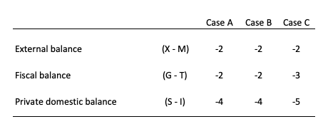
The first two possibilities we might call A and B:

A: A nation can run a current account deficit with an offsetting government sector surplus, while the private domestic sector is spending less than they are earn

B: A nation can run a current account deficit with an offsetting government sector surplus, while the private domestic sector is spending more than they are earning.

So Option A says the private domestic sector is saving overall, whereas Option B say the private domestic sector is dis-saving (and going into increasing indebtedness). These options are captured in the first two columns of the Table.

So the arithmetic example depicts an external sector deficit of 2 per cent of GDP and an offsetting fiscal surplus of 2 per cent of GDP.

You can see that the private sector balance is negative (that is, the sector is spending more than they are earning – Investment is greater than Saving – and has to be equal to 4 per cent of GDP.

Given that the only proposition that can be true is:

B: A nation can run a current account deficit with an offsetting government sector surplus, while the private domestic sector is spending more than they are earning.

Column 2 in the Table captures Option C:

C: A nation can run a current account deficit with a government sector surplus that is larger, while the private domestic sector is spending less than they are earning.

So the current account deficit is equal to 2 per cent of GDP while the surplus is now larger at 3 per cent of GDP. You can see that the private domestic deficit rises to 5 per cent of GDP to satisfy the accounting rule that the balances sum to zero.

The final option available is:

D: None of the above are possible as they all defy the sectoral balances accounting identity.

It cannot be true because as the Table data shows the rule that the sectoral balances add to zero because they are an accounting identity is satisfied in both cases.

So if the G is spending less than it is “earning” and the external sector is adding less income (X) than it is absorbing spending (M), then the other spending components must be greater than total income.

You may wish to read the following blogs for more information:

• Back to basics – aggregate demand drives output
• Stock-flow consistent macro models
• Norway and sectoral balances
• The OECD is at it again!
• Barnaby, better to walk before we run
• Saturday Quiz – June 19, 2010 – answers and discussion

Question 3:

Modern Monetary Theory (MMT) demonstrates that mass unemployment arises from deficient aggregate demand which calls for an increase in the fiscal deficit to correct the deficiency. This observation is totally at odds with the mainstream view that unemployment can be reduced by cutting real wages relative to productivity.

The answer is False.

In this blog post – What causes mass unemployment? – I outline the way aggregate demand failures causes of mass unemployment and use a simple two person economy to demonstrate the point.

I also presented the famous Keynes versus the Classics debate about the role of real wage cuts in stimulating employment that was well rehearsed during the Great Depression.

The debate was multi-dimensioned but the role of wage flexibility was a key aspect. In the classical model of employment determination, which remains the basis of mainstream textbook analysis, cuts in the nominal wage will increase employment because it is considered they will reduce the real wage.

The mainstream textbook model assumes that economies produce under the constraint of the so-called diminishing marginal product of labour. So adding an extra worker will reduce productivity because they assume the available capital that workers get to use is fixed in the short-run.

This assertion which does not stack up in the real world, yields the downward sloping marginal product of labour (the contribution of the last worker to production) relationship in the textbook model. Then profit maximising firms set the marginal product equal to the real wage to determine their employment decisions.

They do this because the marginal product is what the last worker produces (at the margin) and the real wage is what the worker costs in real terms to hire.

So when they have screwed the last bit of production out of the last worker hired and it equals the real wage, they have thus made “real gains” on all previous workers employed and cannot do any better – hence, they are said to have maximised profits.

Labour demand is thus inversely related to the real wage. As the real wage rises, employment falls in this model because the marginal product falls with employment.

The simplest version is that labour supply in the mainstream model (and complex versions don’t add anything anyway) says that households equate the marginal disutility of work (the slope of the labour supply function) with the real wage (indicating the opportunity cost of leisure) to determine their utility maximising labour supply.

So in English, it is assumed that workers hate work and but like leisure (non-work). They will only go to work to get an income and the higher the real wage the more work they will supply because for each hour of labour supplied their prospective income is higher. Again, this conception is arbitrary and not consistent with countless empirical studies which show the total labour supply is more or less invariant to movements in the real wage.

Other more complex variations of the mainstream model depict labour supply functions with both non-zero real wage elasticities and, consistent with recent real business cycle analysis, sensitivity to the real interest rate. All ridiculous. Ignore them!

In the mainstream model, labour market clearing – that is when all firms who want to hire someone can find a worker to hire and all workers who want to work can find sufficient work – requires that the real wage equals the marginal product of labour. The real wage will change to ensure that this is maintained at all times thus providing the classical model with continuous full employment. So anything that prevents this from happening (government regulations) will create unemployment.

If a worker is “unemployed” then it must mean they desire a real wage that is excessive in relation to their productivity. The other way the mainstream characterise this is that the worker values leisure greater than income (work).

The equilibrium employment levels thus determine via the technological state of the economy (productivity function) the equilibrium (or full employment) level of aggregate supply of real output. So once all the labour markets are cleared the total level of output that is produced (determined by the productivity levels) will equal total output or GDP.

It was of particular significance for Keynes that the classical explanation for real output determination did not depend on the aggregate demand for it at all.

He argued that firms will not produce output that they do not think they will sell. So for him, total supply of GDP must be determined by aggregate demand (which he called effective demand – spending plans backed by a willingness to impart cash).

In the General Theory, Keynes questioned whether wage reductions could be readily achieved and was sceptical that, even if they could, employment would rise.

The adverse consequences for the effective demand for output were his principal concern.

So Keynes proposed the revolutionary idea (at the time) that employment was determined by effective monetary demand for output. Since there was no reason why the total demand for output would necessarily correspond to full employment, involuntary unemployment was likely.

Keynes revived Marx’s earlier works on effective demand (although he didn’t acknowledge that in his work – being anti-Marxist). What determined effective demand? There were two major elements: the consumption demand of households, and the investment demands of business.

So demand for aggregate output determined production levels which in turn determined total employment.

Keynes model reversed the classical causality in the macroeconomy. Demand determined output. Production levels then determined employment based on the current level of productivity. The labour market is then constrained by this level of employment demand. At the current money wage level, the level of unemployment (supply minus demand) is then determined. The firms will not expand employment unless the aggregate constraint is relaxed.

Keynes also argued that in a recession, the real wage might not fall because workers bargain for money or nominal wages, not real wages. The act of dropping money wages across the board would also reduce aggregate demand and prices would also fall. So there was no guarantee that real wages (the ratio of wages to prices) would therefore fall. They may rise or stay about the same.

Falling prices might, however, depress business profit expectations and so cut into demand for investment. This would actually reduce the demand for workers and prevent total employment from rising. The system interacts with itself, and an equilibrium of full employment cannot be achieved within the labour market.

Keynes also claimed that in a recession it should be clear that the problem is not that the real wage is too high, but rather that the prices are too low (as prices fall with lower production).

However, in Keynes’ analysis, attempting to cut real wages by cutting nominal wages would be resisted by the workers because they will not promote higher employment or output and also would imperil their ability to service their nominal contractual commitments (like mortgages). The argument is that workers will tolerate a fall in real wages brought about by prices rising faster than nominal wages because, within limits, they can still pay their nominal contractual obligations (by cutting back on other expenditure).

A more subtle point argued by Keynes is that wage cut resistance may be beneficial because of the distribution of income implications. If real wages fall, the share of real output claimed by the owners of capital (or non-labour fixed inputs) rises. Assuming such ownership is concentrated in a few hands, capitalists can be expected to have a higher propensity to save than the working class.

If so, aggregate saving from real output will increase and aggregate demand will fall further setting off a second round of oversupply of output and job losses.

It is also important to differentiate what happens if a firm lowers its wage level against what happens in the whole economy does the same. This relates to the so-called interdependence of demand and supply curves.

The mainstream model claims that the two sides of the market are independent so that a supply shift will not cause the demand side of the market to shift. So in this context, if a firm can lower its money wage rates it would not expect a major fall in the demand for its products because its workforce are a small proportion of total employment and their incomes are a small proportion of total demand.

If so, the firm can reduce its prices and may enjoy rising demand for its output and hence put more workers on. So the demand and supply of output are independent.

However there are solid reasons why firms will not want to behave like this. They get the reputation of being a capricious employer and will struggle to retain labour when the economy improves. Further, worker morale will fall and with it productivity. Other pathologies such as increased absenteeism etc would accompany this sort of firm behaviour.

But if the whole economy takes a wage cut, then while wage are a cost on the supply side they are an income on the demand side. So a cut in wages may reduce supply costs but also will reduce demand for output. In this case the aggregate demand and supply are interdependent and this violates the mainstream depiction.

This argument demonstrates one of the famous fallacies of composition in mainstream theory. That is, policies that might work at the micro (firm/sector) level will not generalise to work at the macroeconomic level.

There was much more to the Keynes versus the Classics debate but the general idea is as presented.

MMT integrates the insights of Keynes and others into a broader monetary framework. But the essential point is that mass unemployment is a macroeconomic phenomenon and trying to manipulate wage levels (relative to prices) will only change output and employment at the macroeconomic level if changes in demand are achieved as saving desires of the non-government sector respond.

It is highly unlikely for all the reasons noted that cutting real wages will reduce the non-government desire to save.

MMT tells us that the introduction of state money (the currency issued by the government) introduces the possibility of unemployment. There is no unemployment in non-monetary economies. As a background to this discussion you might like to read this blog – Functional finance and modern monetary theory .

MMT shows that taxation functions to promote offers from private individuals to government of goods and services in return for the necessary funds to extinguish the tax liabilities.

So taxation is a way that the government can elicit resources from the non-government sector because the latter have to get $s to pay their tax bills. Where else can they get the $s unless the government spends them on goods and services provided by the non-government sector?

A sovereign government is never revenue constrained and so taxation is not required to “finance” public spending. The mainstream economists conceive of taxation as providing revenue to the government which it requires in order to spend. In fact, the reverse is the truth.

Government spending provides revenue to the non-government sector which then allows them to extinguish their taxation liabilities. So the funds necessary to pay the tax liabilities are provided to the non-government sector by government spending.

It follows that the imposition of the taxation liability creates a demand for the government currency in the non-government sector which allows the government to pursue its economic and social policy program.

The non-government sector will seek to sell goods and services (including labour) to the government sector to get the currency (derived from the government spending) in order to extinguish its tax obligations to government as long as the tax regime is legally enforceable. Under these circumstances, the non-government sector will always accept government money because it is the means to get the $s necessary to pay the taxes due.

This insight allows us to see another dimension of taxation which is lost in mainstream economic analysis. Given that the non-government sector requires fiat currency to pay its taxation liabilities, in the first instance, the imposition of taxes (without a concomitant injection of spending) by design creates unemployment (people seeking paid work) in the non-government sector.

The unemployed or idle non-government resources can then be utilised through demand injections via government spending which amounts to a transfer of real goods and services from the non-government to the government sector.

In turn, this transfer facilitates the government’s socio-economics program. While real resources are transferred from the non-government sector in the form of goods and services that are purchased by government, the motivation to supply these resources is sourced back to the need to acquire fiat currency to extinguish the tax liabilities.

Further, while real resources are transferred, the taxation provides no additional financial capacity to the government of issue.
Conceptualising the relationship between the government and non-government sectors in this way makes it clear that it is government spending that provides the paid work which eliminates the unemployment created by the taxes.

So it is now possible to see why mass unemployment arises. It is the introduction of State Money (defined as government taxing and spending) into a non-monetary economy that raises the spectre of involuntary unemployment.

As a matter of accounting, for aggregate output to be sold, total spending must equal the total income generated in production (whether actual income generated in production is fully spent or not in each period).

Involuntary unemployment is idle labour offered for sale with no buyers at current prices (wages). Unemployment occurs when the private sector, in aggregate, desires to earn the monetary unit of account through the offer of labour but doesn’t desire to spend all it earns, other things equal.

As a result, involuntary inventory accumulation among sellers of goods and services translates into decreased output and employment.

In this situation, nominal (or real) wage cuts per se do not clear the labour market, unless those cuts somehow eliminate the private sector desire to net save, and thereby increase spending.

So we are now seeing that at a macroeconomic level, manipulating wage levels (or rates of growth) would not seem to be an effective strategy to solve mass unemployment.

MMT then concludes that mass unemployment occurs when net government spending is too low.

To recap: The purpose of State Money is to facilitate the movement of real goods and services from the non-government (largely private) sector to the government (public) domain.

Government achieves this transfer by first levying a tax, which creates a notional demand for its currency of issue.

To obtain funds needed to pay taxes and net save, non-government agents offer real goods and services for sale in exchange for the needed units of the currency. This includes, of-course, the offer of labour by the unemployed.

The obvious conclusion is that unemployment occurs when net government spending is too low to accommodate the need to pay taxes and the desire to net save.

This analysis also sets the limits on government spending. It is clear that government spending has to be sufficient to allow taxes to be paid. In addition, net government spending is required to meet the private desire to save (accumulate net financial assets).

It is also clear that if the
Government doesn’t spend enough to cover taxes and the non-government sector’s desire to save the manifestation of this deficiency will be unemployment.

Keynesians have used the term demand-deficient unemployment. In MMT, the basis of this deficiency is at all times inadequate net government spending, given the private spending (saving) decisions in force at any particular time.

Shift in private spending certainly lead to job losses but the persistent of these job losses is all down to inadequate net government spending.

But in terms of the question – after all that – it is clear that excessive real wages could impinge on the rate of profit that the capitalists desired and if they translate that into a cut back in investment then aggregate demand might fall. Note: this explanation has nothing to do with the standard mainstream textbook explanation. It is totally consistent with MMT and the Keynesian story – output and employment is determined by aggregate demand and anything that impacts adversely on the latter will undermine employment.

The following blogs may be of further interest to you:

• Functional finance and modern monetary theory
• What causes mass unemployment?
• Modern monetary theory in an open economy
• Deficit spending 101 – Part 1
• Deficit spending 101 – Part 2
• Deficit spending 101 – Part 3

That is enough for today!

(c) Copyright 2019 William Mitchell. All Rights Reserved.