Here are the answers with discussion for this Weekend’s Quiz. The information provided should help you work out why you missed a question or three! If you haven’t already done the Quiz from yesterday then have a go at it before you read the answers. I hope this helps you develop an understanding of Modern…
The Weekend Quiz – June 29-30, 2019 – answers and discussion
Here are the answers with discussion for this Weekend’s Quiz. The information provided should help you work out why you missed a question or three! If you haven’t already done the Quiz from yesterday then have a go at it before you read the answers. I hope this helps you develop an understanding of Modern Monetary Theory (MMT) and its application to macroeconomic thinking. Comments as usual welcome, especially if I have made an error.
Question 1:
The private domestic sector can save overall even if the government fiscal balance is in surplus as long as net exports are positive.
The answer is False.
This is a question about the relative magnitude of the sectoral balances – the government fiscal balance, the external balance and the private domestic balance. The balances taken together always add to zero because they are derived as an accounting identity from the national accounts. The balances reflect the underlying economic behaviour in each sector which is interdependent – given this is a macroeconomic system we are considering.
To refresh your memory the balances are derived as follows. The basic income-expenditure model in macroeconomics can be viewed in (at least) two ways: (a) from the perspective of the sources of spending; and (b) from the perspective of the uses of the income produced. Bringing these two perspectives (of the same thing) together generates the sectoral balances.
From the sources perspective we write:
(1) GDP = C + I + G + (X – M)
which says that total national income (GDP) is the sum of total final consumption spending (C), total private investment (I), total government spending (G) and net exports (X – M).
Expression (1) tells us that total income in the economy per period will be exactly equal to total spending from all sources of expenditure.
We also have to acknowledge that financial balances of the sectors are impacted by net government taxes (T) which includes all tax revenue minus total transfer and interest payments (the latter are not counted independently in the expenditure Expression (1)).
Further, as noted above the trade account is only one aspect of the financial flows between the domestic economy and the external sector. we have to include net external income flows (FNI).
Adding in the net external income flows (FNI) to Expression (2) for GDP we get the familiar gross national product or gross national income measure (GNP):
(2) GNP = C + I + G + (X – M) + FNI
To render this approach into the sectoral balances form, we subtract total net taxes (T) from both sides of Expression (3) to get:
(3) GNP – T = C + I + G + (X – M) + FNI – T
Now we can collect the terms by arranging them according to the three sectoral balances:
(4) (GNP – C – T) – I = (G – T) + (X – M + FNI)
The the terms in Expression (4) are relatively easy to understand now.
The term (GNP – C – T) represents total income less the amount consumed less the amount paid to government in taxes (taking into account transfers coming the other way). In other words, it represents private domestic saving.
The left-hand side of Equation (4), (GNP – C – T) – I, thus is the overall saving of the private domestic sector, which is distinct from total household saving denoted by the term (GNP – C – T).
In other words, the left-hand side of Equation (4) is the private domestic financial balance and if it is positive then the sector is spending less than its total income and if it is negative the sector is spending more than it total income.
The term (G – T) is the government financial balance and is in deficit if government spending (G) is greater than government tax revenue minus transfers (T), and in surplus if the balance is negative.
Finally, the other right-hand side term (X – M + FNI) is the external financial balance, commonly known as the current account balance (CAD). It is in surplus if positive and deficit if negative.
In English we could say that:
The private financial balance equals the sum of the government financial balance plus the current account balance.
We can re-write Expression (6) in this way to get the sectoral balances equation:
(5) (S – I) = (G – T) + CAB
which is interpreted as meaning that government sector deficits (G – T > 0) and current account surpluses (CAB > 0) generate national income and net financial assets for the private domestic sector.
Conversely, government surpluses (G – T < 0) and current account deficits (CAB < 0) reduce national income and undermine the capacity of the private domestic sector to add financial assets.
Expression (5) can also be written as:
(6) [(S – I) – CAB] = (G – T)
where the term on the left-hand side [(S – I) – CAB] is the non-government sector financial balance and is of equal and opposite sign to the government financial balance.
This is the familiar MMT statement that a government sector deficit (surplus) is equal dollar-for-dollar to the non-government sector surplus (deficit).
The sectoral balances equation says that total private savings (S) minus private investment (I) has to equal the public deficit (spending, G minus taxes, T) plus net exports (exports (X) minus imports (M)) plus net income transfers.
All these relationships (equations) hold as a matter of accounting and not matters of opinion.
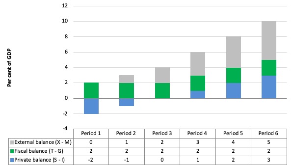
The following graph with accompanying data table lets you see the evolution of the balances expressed in terms of percent of GDP.
In each period I just held the fiscal balance at a constant surplus (2 per cent of GDP) (green bars).
The assumption is artificial because as economic activity changes the automatic stabilisers would lead to endogenous changes in the fiscal balance. But we will just assume there is no change for simplicity. It doesn’t violate the logic.
Also note that I have constructed the graph so that the government balance is expressed as (T – G) so that a surplus is a positive number.
If the nation is running an external surplus it means that the contribution to aggregate demand from the external sector is positive – that is net addition to spending which would increase output and national income.
The external deficit also means that foreigners are decreasing financial claims denominated in the local currency. Given that exports represent a real cost and imports a real benefit, the motivation for a nation running a net exports surplus (the exporting nation in this case) must be to accumulate financial claims (assets) denominated in the currency of the nation running the external deficit.
A fiscal surplus also means the government is spending less than it is “earning” and that puts a drag on aggregate demand and constrains the ability of the economy to grow. So the question is what are the relative magnitudes of the external add and the fiscal subtract from income?
In Period 1, there is an external balance (X – M = 0) and then for each subsequent period the external balance goes into surplus incrementing by 1 per cent of GDP each period (gray bars).
You can see that in the first two periods, overall private domestic saving is negative. As the external surplus is smaller than the fiscal surplus.
Then, as the demand injection from the external surplus offsets the fiscal drag arising from the government surplus, the private domestic sector breakeven (spending as much as they earn, so S – I = 0).
Then the net spending add overall arising from the offsetting positions of the external and public sectors is positive and the income growth would allow the private domestic sector to save overall. That is increasingly so as the net demand add increases with the increasing external surplus.
The following blog posts may be of further interest to you:
- Barnaby, better to walk before we run
- Stock-flow consistent macro models
- Norway and sectoral balances
- The OECD is at it again!
- Saturday Quiz – June 19, 2010 – answers and discussion
Question 2:
The difference between quantitative easing and an increasing fiscal deficit is that the former creates no new net financial assets in the currency of issue.
The answer is True.
Quantitative easing then involves the central bank buying assets from the private sector – government bonds and high quality corporate debt.
So what the central bank is doing is swapping financial assets with the banks – they sell their financial assets and receive back in return extra reserves.
The central bank is thus buying one type of financial asset (private holdings of bonds, company paper) and exchanging it for another (reserve balances at the central bank).
The net financial assets in the private sector are in fact unchanged although the portfolio composition of those assets is altered (maturity substitution) which changes yields and returns.
In terms of changing portfolio compositions, quantitative easing increases central bank demand for “long maturity” assets held in the private sector which reduces interest rates at the longer end of the yield curve.
These are traditionally thought of as the investment rates. This might increase aggregate demand given the cost of investment funds is likely to drop.
But on the other hand, the lower rates reduce the interest-income of savers who will reduce consumption (demand) accordingly.
How these opposing effects balance out is unclear but the evidence suggests there is not very much impact at all.
Expansionary fiscal policy adds net financial assets to the non-government sector by way of contradistinction to QE.
Like all government spending, the Treasury would credit the reserve accounts held by the commercial bank at the central bank. The commercial bank in question would be where the target of the spending had an account. So the commercial bank’s assets rise and its liabilities also increase because a deposit would be made.
The transactions are clear: The commercial bank’s assets rise and its liabilities also increase because a new deposit has been made. Further, the target of the fiscal initiative enjoys increased assets (bank deposit) and net worth (a liability/equity entry on their balance sheet). Taxation does the opposite and so a deficit (spending greater than taxation) means that reserves increase and private net worth increases.
This means that there are likely to be excess reserves in the “cash system” which then raises issues for the central bank about its liquidity management.
But at this stage, M1 (deposits in the non-government sector) rise as a result of the deficit without a corresponding increase in liabilities. In other words, fiscal deficits increase net financial assets in the non-government sector.
What would happen if there were bond sales? All that happens is that the banks reserves are reduced by the bond sales but this does not reduce the deposits created by the net spending.
So net worth is not altered. What is changed is the composition of the asset portfolio held in the non-government sector.
The only difference between the Treasury “borrowing from the central bank” and issuing debt to the private sector is that the central bank has to use different operations to pursue its policy interest rate target.
If it debt is not issued to match the deficit then it has to either pay interest on excess reserves (which most central banks are doing now anyway) or let the target rate fall to zero (the Japan solution).
There is no difference to the impact of the deficits on net worth in the non-government sector.
The following blog posts may be of further interest to you:
- Money multiplier and other myths
- Islands in the sun
- Operation twist – then and now
- Quantitative easing 101
- Building bank reserves will not expand credit
- Building bank reserves is not inflationary
- Deficit spending 101 – Part 1
- Deficit spending 101 – Part 2
- Deficit spending 101 – Part 3
Question 3:
A fiscal deficit that is equivalent to 5 per cent of GDP always signals a more expansionary fiscal intent from government than a deficit outcome that is equivalent to 3 per cent of GDP.
The answer is False.
If I had left the “always” out of the question then the answer would have been Maybe. The inclusion of that more strict requirement (always) renders the proposition false.
The question probes an understanding of the forces (components) that drive the fiscal balance that is reported by government agencies at various points in time.
In outright terms, a fiscal deficit that is equivalent to 5 per cent of GDP is more expansionary than a fiscal deficit outcome that is equivalent to 3 per cent of GDP. But that is not what the question asked. The question asked whether that signalled a more expansionary fiscal intent from government.
In other words, what does the fiscal outcome signal about the discretionary fiscal stance adopted by the government.
To see the difference between these statements we have to explore the issue of decomposing the observed fiscal balance into the discretionary (now called structural) and cyclical components. The latter component is driven by the automatic stabilisers that are in-built into the fiscal process.
The federal (or national) government fiscal balance is the difference between total federal revenue and total federal outlays. So if total revenue is greater than outlays, the fiscal position is in surplus and vice versa. It is a simple matter of accounting with no theory involved. However, the fiscal balance is used by all and sundry to indicate the fiscal stance of the government.
So if the fiscal position is in surplus it is often concluded that the fiscal impact of government is contractionary (withdrawing net spending) and if the fiscal position is in deficit we say the fiscal impact expansionary (adding net spending).
Further, a rising deficit (falling surplus) is often considered to be reflecting an expansionary policy stance and vice versa. What we know is that a rising deficit may, in fact, indicate a contractionary fiscal stance – which, in turn, creates such income losses that the automatic stabilisers start driving the fiscal position back towards (or into) deficit.
So the complication is that we cannot conclude that changes in the fiscal impact reflect discretionary policy changes. The reason for this uncertainty clearly relates to the operation of the automatic stabilisers.
To see this, the most simple model of the fiscal balance we might think of can be written as:
Fiscal balance = Revenue – Spending.
Fiscal balance = (Tax Revenue + Other Revenue) – (Welfare Payments + Other Spending)
We know that Tax Revenue and Welfare Payments move inversely with respect to each other, with the latter rising when GDP growth falls and the former rises with GDP growth. These components of the fiscal balance are the so-called automatic stabilisers.
In other words, without any discretionary policy changes, the fiscal balance will vary over the course of the business cycle. When the economy is weak – tax revenue falls and welfare payments rise and so the fiscal balance moves towards deficit (or an increasing deficit). When the economy is stronger – tax revenue rises and welfare payments fall and the fiscal balance becomes increasingly positive. Automatic stabilisers attenuate the amplitude in the business cycle by expanding the fiscal position in a recession and contracting it in a boom.
So just because the fiscal position goes into deficit or the deficit increases as a proportion of GDP doesn’t allow us to conclude that the Government has suddenly become of an expansionary mind. In other words, the presence of automatic stabilisers make it hard to discern whether the fiscal policy stance (chosen by the government) is contractionary or expansionary at any particular point in time.
To overcome this uncertainty, economists devised what used to be called the ‘Full Employment or High Employment Budget’. In more recent times, this concept is now called the ‘Structural Balance’. The change in nomenclature is very telling because it occurred over the period that neo-liberal governments began to abandon their commitments to maintaining full employment and instead decided to use unemployment as a policy tool to discipline inflation.
The ‘Full Employment Budget Balance’ was a hypothetical construct of the fiscal balance that would be realised if the economy was operating at potential or full employment. In other words, calibrating the fiscal position (and the underlying fiscal parameters) against some fixed point (full capacity) eliminated the cyclical component – the swings in activity around full employment.
So a ‘full employment fiscal’ would be balanced if total outlays and total revenue were equal when the economy was operating at total capacity. If the fiscal position was in surplus at full capacity, then we would conclude that the discretionary structure of the fiscal position was contractionary and vice versa if the fiscal position was in deficit at full capacity.
The calculation of the structural deficit spawned a bit of an industry in the past with lots of complex issues relating to adjustments for inflation, terms of trade effects, changes in interest rates and more.
Much of the debate centred on how to compute the unobserved full employment point in the economy. There were a plethora of methods used in the period of true full employment in the 1960s. All of them had issues but like all empirical work – it was a dirty science – relying on assumptions and simplifications. But that is the nature of the applied economist’s life.
As I explain in the blogs cited below, the measurement issues have a long history and current techniques and frameworks based on the concept of the Non-Accelerating Inflation Rate of Unemployment (the NAIRU) bias the resulting analysis such that actual discretionary positions which are contractionary are seen as being less so and expansionary positions are seen as being more expansionary.
The result is that modern depictions of the structural deficit systematically understate the degree of discretionary contraction coming from fiscal policy.
So the data provided by the question could indicate a more expansionary fiscal intent from government but it could also indicate a large automatic stabiliser (cyclical) component.
Therefore the best answer is false because there are circumstances where the proposition will not hold. It doesn’t always hold.
You might like to read these blog posts for further information:
That is enough for today!
(c) Copyright 2019 William Mitchell. All Rights Reserved.
Does QE run the risk of “bidding up” financial asset classes and therefore increasing private financial assets over a cycle of transactions?
For example, sell bonds at market price X then buy bonds at market price X+1. It seems that financial assets have increased by 1 unit.