Here are the answers with discussion for this Weekend’s Quiz. The information provided should help you work out why you missed a question or three! If you haven’t already done the Quiz from yesterday then have a go at it before you read the answers. I hope this helps you develop an understanding of Modern…
The Weekend Quiz – September 21-22, 2019 – answers and discussion
Here are the answers with discussion for this Weekend’s Quiz. The information provided should help you work out why you missed a question or three! If you haven’t already done the Quiz from yesterday then have a go at it before you read the answers. I hope this helps you develop an understanding of Modern Monetary Theory (MMT) and its application to macroeconomic thinking. Comments as usual welcome, especially if I have made an error.
Question 1:
Some mainstream economists claim that a public debt ratio of 80 per cent is a dangerous threshold that should not be passed. Accordingly, governments should run primary surpluses (taxation revenue in excess of non-interest government spending) to keep the ratio below the threshold. Modern monetary theory tells us that while a currency-issuing government running a deficit can never reduce the debt ratio it doesn’t matter anyway because such a government faces no risk of insolvency.
The answer is False.
While Modern Monetary Theory (MMT) places no particular importance in the public debt to GDP ratio for a sovereign government, given that insolvency is not an issue, the mainstream debate is dominated by the concept.
The unnecessary practice of fiat currency-issuing governments of issuing public debt $-for-$ to match public net spending (deficits) ensures that the debt levels will rise when there are deficits.
Rising deficits usually mean declining economic activity (especially if there is no evidence of accelerating inflation) which suggests that the debt/GDP ratio may be rising because the denominator is also likely to be falling or rising below trend.
Further, historical experience tells us that when economic growth resumes after a major recession, during which the public debt ratio can rise sharply, the latter always declines again.
It is this endogenous nature of the ratio that suggests it is far more important to focus on the underlying economic problems which the public debt ratio just mirrors.
Mainstream economics starts with the flawed analogy between the household and the sovereign government such that any excess in government spending over taxation receipts has to be “financed” in two ways: (a) by borrowing from the public; and/or (b) by “printing money”.
Neither characterisation is remotely representative of what happens in the real world in terms of the operations that define transactions between the government and non-government sector.
Further, the basic analogy is flawed at its most elemental level. The household must work out the financing before it can spend. The household cannot spend first. The government can spend first and ultimately does not have to worry about financing such expenditure.
However, in the mainstream framework for analysing these so-called “financing” choices – the Government Budget Constraint (GBC) – the fiscal deficit in year t is equal to the change in government debt over year t plus the change in high powered money over year t. So in mathematical terms it is written as:
![]()
which you can read in English as saying that Fiscal deficit = Government spending + Government interest payments – Tax receipts must equal (be “financed” by) a change in Bonds (B) and/or a change in high powered money (H). The triangle sign (delta) is just shorthand for the change in a variable.
However, this is merely an accounting statement.
In a stock-flow consistent macroeconomics, this statement will always hold. That is, it has to be true if all the transactions between the government and non-government sector have been corrected added and subtracted.
So in terms of MMT, the previous equation is just an ex post accounting identity that has to be true by definition and has not real economic importance.
But for the mainstream economist, the equation represents an ex ante (before the fact) financial constraint that the government is bound by. The difference between these two conceptions is very significant and the second (mainstream) interpretation cannot be correct if governments issue fiat currency (unless they place voluntary constraints on themselves to act as if it is).
Further, in mainstream economics, money creation is erroneously depicted as the government asking the central bank to buy treasury bonds which the central bank in return then prints money. The government then spends this money. This is called debt monetisation and you can find out why this is typically not a viable option for a central bank by reading the Deficits 101 suite – Deficit spending 101 – Part 1 – Deficit spending 101 – Part 2 – Deficit spending 101 – Part 3.
Anyway, the mainstream claims that if governments increase the money growth rate (they erroneously call this “printing money”) the extra spending will cause accelerating inflation because there will be “too much money chasing too few goods”! Of-course, we know that proposition to be generally preposterous because economies that are constrained by deficient demand (defined as demand below the full employment level) respond to nominal demand increases by expanding real output rather than prices. There is an extensive literature pointing to this result.
So when governments are expanding deficits to offset a collapse in private spending, there is plenty of spare capacity available to ensure output rather than inflation increases.
But not to be daunted by the “facts”, the mainstream claim that because inflation is inevitable if “printing money” occurs, it is unwise to use this option to “finance” net public spending.
Hence they say as a better (but still poor) solution, governments should use debt issuance to “finance” their deficits. Thy also claim this is a poor option because in the short-term it is alleged to increase interest rates and in the longer-term is results in higher future tax rates because the debt has to be “paid back”.
Neither proposition bears scrutiny – you can read these blogs – Will we really pay higher taxes? and Will we really pay higher interest rates? – for further discussion on these points.
The mainstream textbooks are full of elaborate models of debt pay-back, debt stabilisation etc which all claim (falsely) to “prove” that the legacy of past deficits is higher debt and to stabilise the debt, the government must eliminate the deficit which means it must then run a primary surplus equal to interest payments on the existing debt.
A primary fiscal balance is the difference between government spending (excluding interest rate servicing) and taxation revenue.
The standard mainstream framework, which even the so-called progressives (deficit-doves) use, focuses on the ratio of debt to GDP rather than the level of debt per se. The following equation captures the approach:
![]()
So the change in the debt ratio is the sum of two terms on the right-hand side: (a) the difference between the real interest rate (r) and the GDP growth rate (g) times the initial debt ratio; and (b) the ratio of the primary deficit (G-T) to GDP.
The real interest rate is the difference between the nominal interest rate and the inflation rate.
This standard mainstream framework is used to highlight the dangers of running deficits. But even progressives (not me) use it in a perverse way to justify deficits in a downturn balanced by surpluses in the upturn.
The question notes that “some mainstream economists” claim that a ratio of 80 per cent is a dangerous threshold that should not be passed – this is the Reinhart and Rogoff story.
Many mainstream economists and a fair number of so-called progressive economists say that governments should as some point in the business cycle run primary surpluses (taxation revenue in excess of non-interest government spending) to start reducing the debt ratio back to “safe” territory.
Almost all the media commentators that you read on this topic take it for granted that the only way to reduce the public debt ratio is to run primary surpluses. That is what the whole “credible exit strategy” hoopla is about.
Further, there is no analytical definition ever provided of what safe is and fiscal rules such as those imposed on the Eurozone nations by the Stability and Growth Pact (a maximum public debt ratio of 60 per cent) are totally arbitrary and without any foundation at all. Just numbers plucked out of the air by those who do not understand the monetary system.
But the specific question you had to respond to (TRUE/FALSE) after some background information was:
Modern monetary theory tells us that while a currency-issuing government running a deficit can never reduce the debt ratio it doesn’t matter anyway because such a government faces no risk of insolvency.
MMT does not tell us that a currency-issuing government running a deficit can never reduce the debt ratio. That was the falsehood that made the correct answer false. The other part of that sentence is true but was designed to lull you into incorrect analytical thinking.
The standard formula above can easily demonstrate that a nation running a primary deficit can reduce its public debt ratio over time.
Furthermore, depending on contributions from the external sector, a nation running a deficit will more likely create the conditions for a reduction in the public debt ratio than a nation that introduces an austerity plan aimed at running primary surpluses.
Here is why that is the case.
A growing economy can absorb more debt and keep the debt ratio constant or falling. From the formula above, if the primary fiscal balance is zero, public debt increases at a rate r but the public debt ratio increases at r – g.
To make matters simple, assume a public debt ratio at the start of the period of 100 per cent (so B/Y(-1) = 1) and a current real interest rate (r) of 3 per cent. Assume that GDP is growing (g) at 2 per cent. This would require a primary surplus of 1 per cent of GDP to stabilise the debt ratio (check it for yourself).
Now what if the financial markets want a risk premium on domestic bonds? Also assume the central bank is worried about inflation and pushes nominal interest rates up so that the real rate (r) rises to 6 per cent. Also assume that the primary surplus and the rising interest rates drive g to 0 per cent (GDP growth falls to zero).
So now the the fiscal austerity (primary surplus) has to rise to 6 per cent of GDP to stabilise debt. The sharp fiscal contraction would lead to recession and as the popularity of the government wanes the uncertainty drives further interest rate rises (via the “markets”). It becomes even harder to stabilise debt as r rises and g falls.
But consider this example which is captured in Year 1 in the Table below. Assume, as before that B/Y(-1) = 1 (that is, the public debt ratio at the start of the period is 100 per cent). The (-1) just signals the value inherited in the current period.
It is a highly stylised example truncated into a two-period adjustment to demonstrate the point. But if the fiscal deficit is a large percentage of GDP then it might take some years to start reducing the public debt ratio as GDP growth ensures.
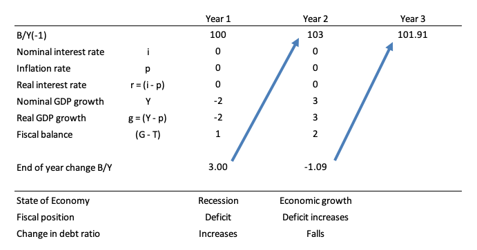
Assume that the real rate of interest is 0 (so the nominal interest rate equals the inflation rate) – not to dissimilar to the situation at present in many countries.
Assume that the rate of real GDP growth is minus 2 per cent (that is, the nation is in recession) and the automatic stabilisers push the primary fiscal balance into deficit equal to 1 per cent of GDP. As a consequence, the public debt ratio will rise by 3 per cent.
The government reacts to the recession in the correct manner and increases its discretionary net spending to take the deficit in Year 2 to 2 per cent of GDP (noting a positive number in this instance is a deficit).
The central bank maintains its zero interest rate policy and the inflation rate also remains at zero.
The increasing deficit stimulates economic growth in Year 2 such that real GDP grows by 3 per cent. In this case the public debt ratio falls by 1.09 per cent.
So even with an increasing (or unchanged) deficit, real GDP growth can reduce the public debt ratio, which is what has happened many times in past history following economic slowdowns.
Economists like Krugman and Mankiw argue that the government could (should) reduce the ratio by inflating it away. Noting that nominal GDP is the product of the price level (P) and real output (Y), the inflating story just increases the nominal value of output and so the denominator of the public debt ratio grows faster than the numerator.
But stimulating real growth (that is, in Y) is the other more constructive way of achieving the same relative adjustment in the denominator of the public debt ratio and its numerator.
But the best way to reduce the public debt ratio is to stop issuing debt. A sovereign government doesn’t have to issue debt if the central bank is happy to keep its target interest rate at zero or pay interest on excess reserves.
The discussion also demonstrates why tightening monetary policy makes it harder for the government to reduce the public debt ratio – which, of-course, is one of the more subtle mainstream ways to force the government to run surpluses.
Question 2:
Imagine that macroeconomic policy is geared towards keeping real GDP growth on trend. Assume this rate of growth is 3 per cent per annum. If labour productivity is growing at 2 per cent per annum and the labour force is growing at 1.5 per cent per annum and the average working week is constant in hours, then this policy regime will result in:
(a) a rising unemployment rate.
(b) a rising unemployment rate.
(c) an unchanged unemployment rate.
The answer is Option (a) a rising unemployment rate.
The facts were:
- Real GDP growth to be maintained at its trend growth rate of 3 per cent annum.
- Labour productivity growth (that is, growth in real output per person employed) growing at 2 per cent per annum. So as this grows less employment in required per unit of output.
- The labour force is growing by 1.5 per cent per annum. Growth in the labour force adds to the employment that has to be generated for unemployment to stay constant (or fall).
- The average working week is constant in hours. So firms are not making hours adjustments up or down with their existing workforce. Hours adjustments alter the relationship between real GDP growth and persons employed.
Of-course, the trend rate of real GDP growth doesn’t relate to the labour market in any direct way. The late Arthur Okun is famous (among other things) for estimating the relationship that links the percentage deviation in real GDP growth from potential to the percentage change in the unemployment rate – the so-called Okun’s Law.
The algebra underlying this law can be manipulated to estimate the evolution of the unemployment rate based on real output forecasts.
From Okun, we can relate the major output and labour-force aggregates to form expectations about changes in the aggregate unemployment rate based on output growth rates. A series of accounting identities underpins Okun’s Law and helps us, in part, to understand why unemployment rates have risen.
Take the following output accounting statement:
(1) Y = LP*(1-UR)LH
where Y is real GDP, LP is labour productivity in persons (that is, real output per unit of labour), H is the average number of hours worked per period, UR is the aggregate unemployment rate, and L is the labour-force. So (1-UR) is the employment rate, by definition.
Equation (1) just tells us the obvious – that total output produced in a period is equal to total labour input [(1-UR)LH] times the amount of output each unit of labour input produces (LP).
Using some simple calculus you can convert Equation (1) into an approximate dynamic equation expressing percentage growth rates, which in turn, provides a simple benchmark to estimate, for given labour-force and labour productivity growth rates, the increase in output required to achieve a desired unemployment rate.
Accordingly, with small letters indicating percentage growth rates and assuming that the average number of hours worked per period is more or less constant, we get:
(2) y = lp + (1 – ur) + lf
Re-arranging Equation (2) to express it in a way that allows us to achieve our aim (re-arranging just means taking and adding things to both sides of the equation):
(3) ur = 1 + lp + lf – y
Equation (3) provides the approximate rule of thumb – if the unemployment rate is to remain constant, the rate of real output growth must equal the rate of growth in the labour-force plus the growth rate in labour productivity.
It is an approximate relationship because cyclical movements in labour productivity (changes in hoarding) and the labour-force participation rates can modify the relationships in the short-run. But it provides reasonable estimates of what happens when real output changes.
The sum of labour force and productivity growth rates is referred to as the required real GDP growth rate – required to keep the unemployment rate constant.
Remember that labour productivity growth (real GDP per person employed) reduces the need for labour for a given real GDP growth rate while labour force growth adds workers that have to be accommodated for by the real GDP growth (for a given productivity growth rate).
So in the example, the required real GDP growth rate is 3.5 per cent per annum and if policy only aspires to keep real GDP growth at its trend growth rate of 3 per cent annum, then the output gap that emerges is 0.5 per cent per annum.
The unemployment rate will rise by this much (give or take) and reflects the fact that real output growth is not strong enough to both absorb the new entrants into the labour market and offset the employment losses arising from labour productivity growth.
Please read my blog – What do the IMF growth projections mean? – for more discussion on this point.
The question has practical relevance in Australia at present with the recent statement by the RBA that its was hiking rates further because real GDP growth was nearly back on trend. The fact is that the trend growth rate is below the required growth rate and so the monetary policy stance is really locking in higher than necessary unemployment.
Question 3:
Students are taught that the macroeconomic income determination system can be thought of as a bath tub with the current GDP being the water level. The drain plug can be thought of as saving, imports and taxation payments (the so-called leakages from the expenditure system) while the taps can be thought of as investment, government spending and exports (the so-called exogenous injections into the spending system). This analogy is valid because GDP will be unchanged as long as the flows into the bath are equal to the flows out of it which is tantamount to saying the the spending gap left by the leakages is always filled by the injections.
The answer is False.
This is actually an example that has been used in the past by macroeconomics teachers to try to teach students the so-called circular expenditure models with leakages and injections.
The basic flaw is that it confuses stocks and flows. It is crucial to a wider understanding of macroeconomics that the distinction between the two concepts is clear in your mind.
The taps and the drains are conceptually accurate because they relate to flows – all expenditure components, saving and taxation payments are flows which are measures as so many $s per period.
A stock has no such time dimension and the only way we can measure it is to take a snapshot at some point in time.
The flaw then relates to the construction of GDP as the level of water in the bath. This is a stock rather than a flow. In the same way as a reservoir is a storage of water which might be 70 or 80 percent full.
But GDP is just the summation of the expenditure flows and is thus a flow itself.
When the national statistician releases the National Accounts and says that GDP was $x billion in the December quarter, they are referring to the sum total of the flow of component expenditure over the 3 month period (October, November, December). They are not referring to a stock of output (which would be inventories or something like that).
The aspect of the question that is true, however, relates to the statement that GDP will be unchanged as long as the flows into the bath are equal to the flows out of it which is tantamount to saying the the spending gap left by the leakages is always filled by the injections.
However the nuance is that it will be the flow of GDP that will be unchanged. The water level is a poor construction of this flow concept.
If we wanted to be aquatic, it would be better to think about a river flowing along with tributaries flowing in and out which alter the water level as it flows along.
That is enough for today!
(c) Copyright 2019 William Mitchell. All Rights Reserved.
In Q2 – option a) and b) are the same.