Here are the answers with discussion for this Weekend’s Quiz. The information provided should help you work out why you missed a question or three! If you haven’t already done the Quiz from yesterday then have a go at it before you read the answers. I hope this helps you develop an understanding of Modern…
The Weekend Quiz – July 25-26, 2020 – answers and discussion
Here are the answers with discussion for this Weekend’s Quiz. The information provided should help you work out why you missed a question or three! If you haven’t already done the Quiz from yesterday then have a go at it before you read the answers. I hope this helps you develop an understanding of Modern Monetary Theory (MMT) and its application to macroeconomic thinking. Comments as usual welcome, especially if I have made an error.
Question 1:
The difference between a situation where the government runs a deficit and matches it with debt-issuance to the non-government sector to a situation where debt is only issued to the central bank is that non-government sector wealth rises in the first case.
The answer is False.
Within a fiat monetary system we need to understand the banking operations that occur when governments spend and issue debt. That understanding allows us to appreciate what would happen if a sovereign, currency-issuing government (with a flexible exchange rate) ran a fiscal deficit without issuing debt?
The question lures you into thinking it is the bond-issuance that drives the rise in non-government net financial wealth when, in fact, it is the fiscal deficit that adds to non-government wealth irrespective of whether bonds are issued or not.
Like all government spending, the Treasury would instruct the central bank to credit the reserve accounts held by the commercial bank at the central bank. The commercial bank in question would be where the target of the spending had an account. So the commercial bank’s assets rise and its liabilities also increase because a deposit would be made.
The transactions are clear: The commercial bank’s assets rise and its liabilities also increase because a new deposit has been made. Further, the target of the fiscal initiative enjoys increased assets (bank deposit) and net worth (a liability/equity entry on their balance sheet). Taxation does the opposite and so a deficit (spending greater than taxation) means that reserves increase and private net worth increases.
This means that there are likely to be excess reserves in the “cash system” which then raises issues for the central bank about its liquidity management. But at this stage, M1 (deposits in the non-government sector) rise as a result of the deficit without a corresponding increase in liabilities. In other words, fiscal deficits increase net financial assets in the non-government sector.
What would happen if there were bond sales? All that happens is that the banks reserves are reduced by the bond sales but this does not reduce the deposits created by the net spending. So net worth is not altered. What is changed is the composition of the asset portfolio held in the non-government sector.
The only difference between the Treasury “borrowing from the central bank” and issuing debt to the private sector is that the central bank has to use different operations to pursue its policy interest rate target.
If debt is not issued to match the deficit then it has to either pay interest on excess reserves (which most central banks are doing now anyway) or let the target rate fall to zero (the Japan solution).
There is no difference to the impact of the deficits on net worth in the non-government sector.
You may wish to read the following blog posts for more information:
- Why history matters
- Building bank reserves will not expand credit
- Building bank reserves is not inflationary
- The complacent students sit and listen to some of that
- Saturday Quiz – February 27, 2010 – answers and discussion
Question 2:
If net exports are running at 2 per cent of GDP, and the private domestic sector overall is saving an equivalent of 3 per cent of GDP, the government must be running a surplus equal to 1 per cent of GDP.
The answer is False.
The correct answer is that the government must be running a deficit equal to 1 per cent of GDP.
To refresh your memory the sectoral balances are derived as follows. The basic income-expenditure model in macroeconomics can be viewed in (at least) two ways: (a) from the perspective of the sources of spending; and (b) from the perspective of the uses of the income produced. Bringing these two perspectives (of the same thing) together generates the sectoral balances.
From the sources perspective we write:
GDP = C + I + G + (X – M)
which says that total national income (GDP) is the sum of total final consumption spending (C), total private investment (I), total government spending (G) and net exports (X – M).
Expression (1) tells us that total income in the economy per period will be exactly equal to total spending from all sources of expenditure.
We also have to acknowledge that financial balances of the sectors are impacted by net government taxes (T) which includes all taxes and transfer and interest payments (the latter are not counted independently in the expenditure Expression (1)).
Further, as noted above the trade account is only one aspect of the financial flows between the domestic economy and the external sector. we have to include net external income flows (FNI).
Adding in the net external income flows (FNI) to Expression (2) for GDP we get the familiar gross national product or gross national income measure (GNP):
(2) GNP = C + I + G + (X – M) + FNI
To render this approach into the sectoral balances form, we subtract total taxes and transfers (T) from both sides of Expression (3) to get:
(3) GNP – T = C + I + G + (X – M) + FNI – T
Now we can collect the terms by arranging them according to the three sectoral balances:
(4) (GNP – C – T) – I = (G – T) + (X – M + FNI)
The the terms in Expression (4) are relatively easy to understand now.
The term (GNP – C – T) represents total income less the amount consumed less the amount paid to government in taxes (taking into account transfers coming the other way). In other words, it represents private domestic saving.
The left-hand side of Equation (4), (GNP – C – T) – I, thus is the overall saving of the private domestic sector, which is distinct from total household saving denoted by the term (GNP – C – T).
In other words, the left-hand side of Equation (4) is the private domestic financial balance and if it is positive then the sector is spending less than its total income and if it is negative the sector is spending more than it total income.
The term (G – T) is the government financial balance and is in deficit if government spending (G) is greater than government tax revenue minus transfers (T), and in surplus if the balance is negative.
Finally, the other right-hand side term (X – M + FNI) is the external financial balance, commonly known as the current account balance (CAD). It is in surplus if positive and deficit if negative.
In English we could say that:
The private financial balance equals the sum of the government financial balance plus the current account balance.
We can re-write Expression (6) in this way to get the sectoral balances equation:
(5) (S – I) = (G – T) + CAB
which is interpreted as meaning that government sector deficits (G – T > 0) and current account surpluses (CAB > 0) generate national income and net financial assets for the private domestic sector.
Conversely, government surpluses (G – T < 0) and current account deficits (CAB < 0) reduce national income and undermine the capacity of the private domestic sector to add financial assets.
Expression (5) can also be written as:
(6) [(S – I) – CAB] = (G – T)
where the term on the left-hand side [(S – I) – CAB] is the non-government sector financial balance and is of equal and opposite sign to the government financial balance.
This is the familiar MMT statement that a government sector deficit (surplus) is equal dollar-for-dollar to the non-government sector surplus (deficit).
The sectoral balances equation says that total private savings (S) minus private investment (I) has to equal the public deficit (spending, G minus taxes, T) plus net exports (exports (X) minus imports (M)) plus net income transfers.
All these relationships (equations) hold as a matter of accounting and not matters of opinion.
Thus, when an external deficit (X – M < 0) and public surplus (G – T < 0) coincide, there must be a private deficit. While private spending can persist for a time under these conditions using the net savings of the external sector, the private sector becomes increasingly indebted in the process.
Second, you then have to appreciate the relative sizes of these balances to answer the question correctly.
The rule is that the sectoral balances have to sum to zero. So if we write the condition above as:
(S – 1) – (G – T) – (X – M) = 0
And substitute the values of the question we get:
3 – (G – T) – 2 = 0
We can solve this for (G – T) as
(G – T) = 3 – 2 = 1
Given the construction (G – T) a positive number (1) is a deficit.
This tells us that even if the external sector is growing strongly and is in surplus there may still be a need for public deficits. This will occur if the private domestic sector seek to save at a proportion of GDP higher than the external surplus.
The economics of this situation might be something like this. The external surplus would be adding to overall aggregate demand (the injection from exports exceeds the drain from imports). However, if the drain from private sector spending (S > I) is greater than the external injection then the only way output and income can remain constant is if the government is in deficit.
National income adjustments would occur if the private domestic sector tried to push for higher saving overall – income would fall (because overall spending fell) and the government would be pushed into deficit whether it liked it or not via falling revenue and rising welfare payments.
You may wish to read the following blog posts for more information:
- Back to basics – aggregate demand drives output
- Stock-flow consistent macro models
- Norway and sectoral balances
- The OECD is at it again!
- Barnaby, better to walk before we run
- Saturday Quiz – June 19, 2010 – answers and discussion
Question 2
To reduce the public debt ratio, the government has to eventually run primary fiscal surpluses (that is, spend less than they raise in taxes net of interest payments on past debt).
The answer is False.
This question requires you to understand the key parameters and relationships that determine the dynamics of the public debt ratio. An understanding of these relationships allows you to debunk statements that are made by those who think fiscal austerity will allow a government to reduce its public debt ratio.
It also requires you to differentiate between the level of outstanding public debt and the ratio of public debt to GDP. The question is focusing on the latter concept.
While Modern Monetary Theory (MMT) places no particular importance in the public debt to GDP ratio for a sovereign government, given that insolvency is not an issue, the mainstream debate is dominated by the concept.
The unnecessary practice of fiat currency-issuing governments of issuing public debt $-for-$ to match public net spending (deficits) ensures that the debt levels will rise when there are deficits.
Rising deficits usually mean declining economic activity (especially if there is no evidence of accelerating inflation) which suggests that the debt/GDP ratio may be rising because the denominator is also likely to be falling or rising below trend.
Further, historical experience tells us that when economic growth resumes after a major recession, during which the public debt ratio can rise sharply, the latter always declines again.
It is this endogenous nature of the ratio that suggests it is far more important to focus on the underlying economic problems which the public debt ratio just mirrors.
Mainstream economics starts with the flawed analogy between the household and the sovereign government such that any excess in government spending over taxation receipts has to be “financed” in two ways: (a) by borrowing from the public; and/or (b) by “printing money”.
Neither characterisation is remotely representative of what happens in the real world in terms of the operations that define transactions between the government and non-government sector.
Further, the basic analogy is flawed at its most elemental level. The household must work out the financing before it can spend. The household cannot spend first. The government can spend first and ultimately does not have to worry about financing such expenditure.
However, the mainstream framework for analysing these so-called “financing” choices is called the government budget constraint (GBC). The GBC says that the fiscal deficit in year t is equal to the change in government debt over year t plus the change in high powered money over year t. So in mathematical terms it is written as:
![]()
which you can read in English as saying that fiscal deficit = government spending + government interest payments – tax receipts must equal (be “financed” by) a change in bonds (B) and/or a change in high powered money (H). The triangle sign (delta) is just shorthand for the change in a variable.
However, this is merely an accounting statement. In a stock-flow consistent macroeconomics, this statement will always hold. That is, it has to be true if all the transactions between the government and non-government sector have been corrected added and subtracted.
So in terms of MMT, the previous equation is just an ex post accounting identity that has to be true by definition and has not real economic importance.
But for the mainstream economist, the equation represents an ex ante (before the fact) financial constraint that the government is bound by. The difference between these two conceptions is very significant and the second (mainstream) interpretation cannot be correct if governments issue fiat currency (unless they place voluntary constraints on themselves to act as if it is).
Further, in mainstream economics, money creation is erroneously depicted as the government asking the central bank to buy treasury bonds which the central bank in return then prints money. The government then spends this money.
This is called debt monetisation and you can find out why this is typically not a viable option for a central bank by reading the Deficits 101 suite – Deficit spending 101 – Part 1 – Deficit spending 101 – Part 2 – Deficit spending 101 – Part 3.
Anyway, the mainstream claims that if governments increase the money growth rate (they erroneously call this “printing money”) the extra spending will cause accelerating inflation because there will be “too much money chasing too few goods”! Of-course, we know that proposition to be generally preposterous because economies that are constrained by deficient demand (defined as demand below the full employment level) respond to nominal demand increases by expanding real output rather than prices. There is an extensive literature pointing to this result.
So when governments are expanding deficits to offset a collapse in private spending, there is plenty of spare capacity available to ensure output rather than inflation increases.
But not to be daunted by the “facts”, the mainstream claim that because inflation is inevitable if “printing money” occurs, it is unwise to use this option to “finance” net public spending.
Hence they say as a better (but still poor) solution, governments should use debt issuance to “finance” their deficits. Thy also claim this is a poor option because in the short-term it is alleged to increase interest rates and in the longer-term is results in higher future tax rates because the debt has to be “paid back”.
Neither proposition bears scrutiny – you can read these blogs – Will we really pay higher taxes? and Will we really pay higher interest rates? – for further discussion on these points.
The mainstream textbooks are full of elaborate models of debt pay-back, debt stabilisation etc which all claim (falsely) to “prove” that the legacy of past deficits is higher debt and to stabilise the debt, the government must eliminate the deficit which means it must then run a primary surplus equal to interest payments on the existing debt.
A primary fiscal balance is the difference between government spending (excluding interest rate servicing) and taxation revenue.
The standard mainstream framework, which even the so-called progressives (deficit-doves) use, focuses on the ratio of debt to GDP rather than the level of debt per se. The following equation captures the approach:
![]()
So the change in the debt ratio is the sum of two terms on the right-hand side: (a) the difference between the real interest rate (r) and the real GDP growth rate (g) times the initial debt ratio; and (b) the ratio of the primary deficit (G-T) to GDP.
The real interest rate is the difference between the nominal interest rate and the inflation rate. Real GDP is the nominal GDP deflated by the inflation rate. So the real GDP growth rate is equal to the Nominal GDP growth minus the inflation rate.
An appreciation of the elements of the public debt ratio immediately tells us that a currency-issuing government running a deficit can reduce the debt ratio. There is no need to run primary surpluses and unnecessarily reduce growth. The standard formula above can easily demonstrate that a nation running a primary deficit can reduce its public debt ratio over time.
Furthermore, depending on contributions from the external sector, a nation running a deficit will more likely create the conditions for a reduction in the public debt ratio than a nation that introduces an austerity plan aimed at running primary surpluses.
Here is why that is the case.
A growing economy can absorb more debt and keep the debt ratio constant or falling. From the formula above, if the primary fiscal balance is zero, public debt increases at a rate r but the public debt ratio increases at r – g.
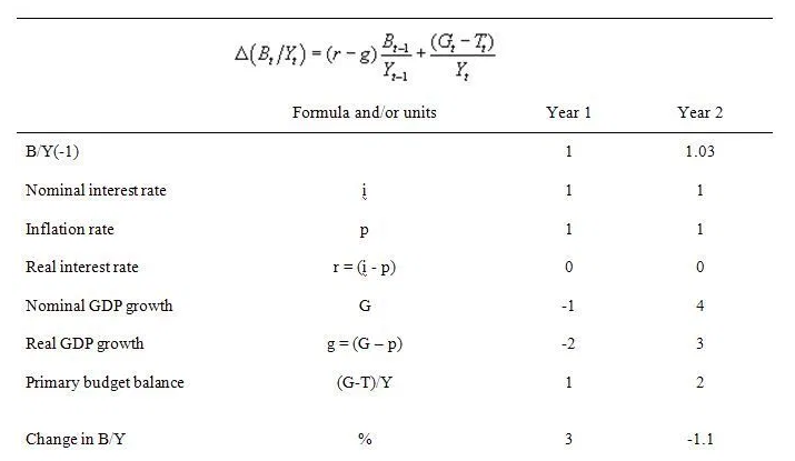
The following Table simulates the two years in question. To make matters simple, assume a public debt ratio at the start of the Year 1 of 100 per cent (so B/Y(-1) = 1) which is equivalent to the statement that “outstanding public debt is equal to the value of the nominal GDP”.
Also the nominal interest rate is 1 per cent and the inflation rate is 1 per cent then the current real interest rate (r) is 0 per cent.
If the nominal GDP is growing at -1 per cent and there is an inflation rate of 1 per cent then real GDP is growing (g) at minus 2 per cent.
Under these conditions, the primary fiscal surplus would have to be equal to 2 per cent of GDP to stabilise the debt ratio (check it for yourself). So, the question suggests the primary fiscal deficit is actually 1 per cent of GDP we know by computation that the public debt ratio rises by 3 per cent.
The calculation (using the formula in the Table) is:
Change in B/Y = (0 – (-2))*1 + 1 = 3 per cent.
The data in Year 2 is given in the last column in the Table below. Note the public debt ratio has risen to 1.03 because of the rise from last year. You are told that the fiscal deficit doubles as per cent of GDP (to 2 per cent) and nominal GDP growth shoots up to 4 per cent which means real GDP growth (given the inflation rate) is equal to 3 per cent.
The corresponding calculation for the change in the public debt ratio is:
Change in B/Y = (0 – 3)*1.03 + 2 = -1.1 per cent.
So the growth in the economy is strong enough to reduce the public debt ratio even though the primary fiscal deficit has doubled.
It is a highly stylised example truncated into a two-period adjustment to demonstrate the point. In the real world, if the fiscal deficit is a large percentage of GDP then it might take some years to start reducing the public debt ratio as GDP growth ensures.
Summary:
Year 1:
– Debt ratio rises.
– Fiscal deficit.
– Recession.
Year 2:
– Debt ratio falls.
– Fiscal deficit rises.
– Economic growth.
So even with an increasing (or unchanged) deficit, real GDP growth can reduce the public debt ratio, which is what has happened many times in past history following economic slowdowns.
The best way to reduce the public debt ratio is to stop issuing debt. A sovereign government doesn’t have to issue debt if the central bank is happy to keep its target interest rate at zero or pay interest on excess reserves.
The discussion also demonstrates why tightening monetary policy makes it harder for the government to reduce the public debt ratio – which, of-course, is one of the more subtle mainstream ways to force the government to run surpluses.
That is enough for today!
(c) Copyright 2020 William Mitchell. All Rights Reserved.
Q2.
Prof. Mitchell concludes (penultimate paragraph) “The best way to reduce the public debt ratio is to stop issuing debt”.
In addition, and more rapid, the debt can be reduced by open-market purchases of government bonds, i.e. debt redemptions prior to the maturity of bonds.
However, as emphasised Abba Lerner in his Principles of Functional Finance, the level of the debt should never be a target of government policies:
“The size of the stock of money as well as the size of the national debt are results of the actions that will have to be undertaken to prevent inflation and deflation and are never considerations that should prevent the government buying and selling, giving and taking, and borrowing and lending”
Lerner – “The Economics of Employment”, 1951, chapter 8